Modeling and Accounting for LD Reference Mismatch in Summary Statistics Fine-mapping

This vignette gives a practical workflow for using susie_rss when the GWAS summary statistics and the supplied LD from external reference samples mismatch, inducing high false positives in fine-mapping. This vignette complements the summary statistics vignette and the older RSS diagnostic vignette.

Because an effect variant induces marginal associations at correlated variants due to LD, SuSiE-RSS uses the input LD matrix to subtract the expected contribution of the fitted effect across the region at each single effect update. If that LD matrix mismatches, the subtraction is imperfect. The leftover residual can then surface as additional sparse association signals, creating spurious additional association signals. The model introduced here targets a specific mechanism by which LD mismatch affects SuSiE-RSS: when the LD matrix is estimated from a finite genotype reference panel, or from a reference panel whose population differs from the target GWAS population.

The approach here is to detect this LD mismatch pattern, quantify the uncertainty it introduces, and attenuate signals that depend strongly on uncertain LD subtraction. In the current susie_rss implementation, R_finite accounts for finite LD reference panel uncertainty, and R_mismatch = "eb" estimates additional LD mismatch component — mainly motivated as population drift — from the data. A separate diagnostic flags the reliability of fine-mapped CS as well as the region by measuring signal attenuation and residual artifacts to caution users to inspect the results.

library(susieR)

count_cs <- function(fit) {
  if (is.null(fit$sets) || is.null(fit$sets$cs)) return(0L)
  length(fit$sets$cs)
}

Recap: a “preventable” allele coding artifact

The older RSS diagnostic vignette discusses allele coding artifacts as source of LD mismatch — specifically the “allele flip”. We briefly revisit the same idea here because it provides a useful contrast with the our finite reference and population-drift LD mismatch model developed below.

data(SummaryConsistency, package = "susieR")
if (!exists("SummaryConsistency"))
  load(file.path("..", "data", "SummaryConsistency.RData"))

zflip <- SummaryConsistency$z
Rtoy <- SummaryConsistency$ldref
flip_id <- SummaryConsistency$flip_id
signal_id <- SummaryConsistency$signal_id
ntoy <- 10000
btoy <- numeric(length(zflip))
btoy[signal_id] <- zflip[signal_id]

With the allele coding problem present, ordinary susie_rss reports the true signal and an additional signal at the mismatched variant.

fit_toy_bad <- susie_rss(zflip, Rtoy, n = ntoy)
# HINT: Setting max_iter = 50 for the SuSiE RSS model because slow convergence is often a sign of unstable summary-statistics fitting. To disable this message, explicitly set max_iter = 50 or another value in the susie_rss() call.
susie_plot(fit_toy_bad, y = "PIP", b = btoy, add_legend = TRUE,
           main = "with allele coding artifact")
points(SummaryConsistency$flip_id,
       fit_toy_bad$pip[flip_id], col = 7, pch = 16)

The kriging diagnostic for allele flip highlights the discordant variant.

kr_toy <- kriging_rss(zflip, Rtoy, n = ntoy)
kr_toy$plot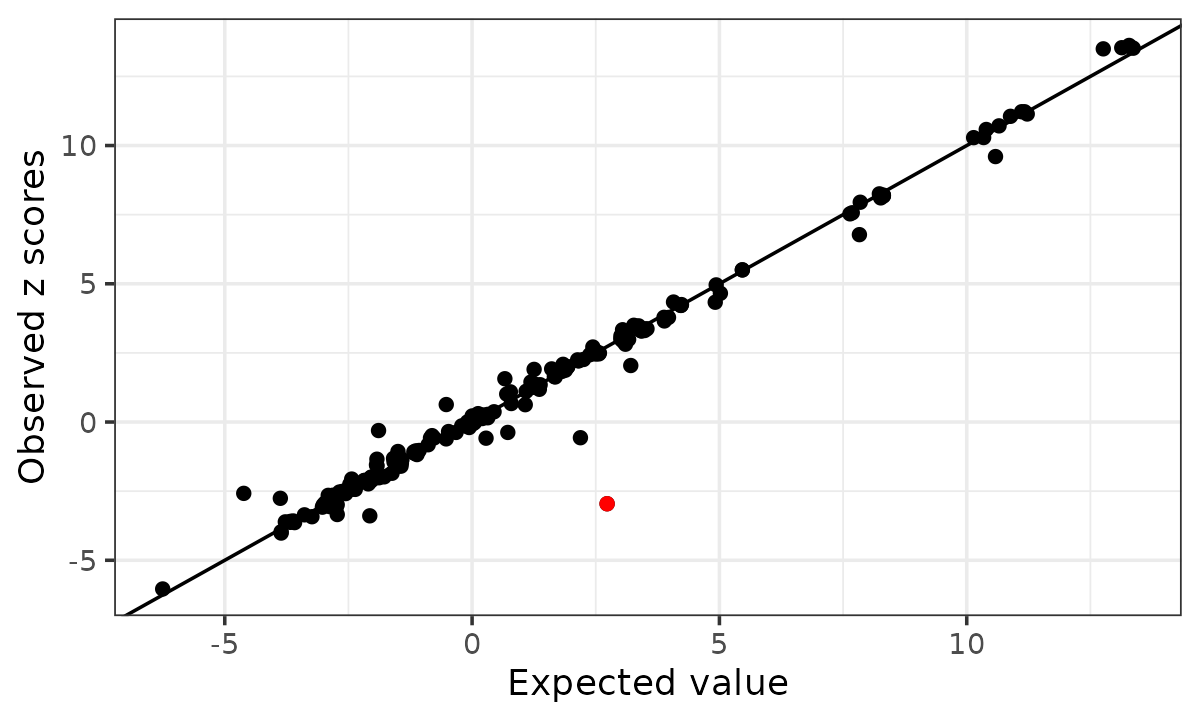

After correcting that allele encoding, the extra credible set disappears.

zfix <- zflip
zfix[flip_id] <- -zfix[flip_id]
fit_toy_fixed <- susie_rss(zfix, Rtoy, n = ntoy)
# HINT: Setting max_iter = 50 for the SuSiE RSS model because slow convergence is often a sign of unstable summary-statistics fitting. To disable this message, explicitly set max_iter = 50 or another value in the susie_rss() call.
susie_plot(fit_toy_fixed, y = "PIP", b = btoy, add_legend = TRUE,
           main = "after allele correction")

In practice, it is useful to run this basic check before modeling LD mismatch. When there is an obvious low level allele coding artifact, it is the best practice to fix it directly through proper bioinformatics procedures. This can be done using many bioinformatics tools, for example pecotmr::allele_qc from this package. In this toy example, susie_rss reports 2 credible sets before the correction and 1 after the correction, and the kriging rule identifies the deliberately misaligned variant.

Example using real GWAS data and a 1000 Genomes European LD reference panel

The example below from real data below shows a different situation where the kriging outlier check does not find isolated variants to remove, but model-based LD uncertainty still changes the fine-mapping result. The summary statistics came from a real GWAS study of a genomic region. The supplied LD matrix R was computed from a 1000 Genomes European LD reference panel with roughly 500 samples. The full region used in the original analysis contains more than 5,000 variants.

In the full region, ordinary susie_rss reported 29 credible sets, whereas setting R_finite = 500 reduced this to 3 credible sets, and adding R_mismatch = "eb" reduced it to 1 credible set. To keep the vignette small, the example included here uses a subset of 500 variants. The rest of this vignette walks through this smaller example step by step, showing how to use R_finite, R_mismatch, and the accompanying diagnostics to evaluate LD mismatch in practice.

data(rss_mismatch_example, package = "susieR")
if (!exists("rss_mismatch_example"))
  load(file.path("..", "data", "rss_mismatch_example.RData"))
z <- rss_mismatch_example$z
bhat <- rss_mismatch_example$bhat
shat <- rss_mismatch_example$shat
n <- rss_mismatch_example$n
R <- rss_mismatch_example$R
str(rss_mismatch_example)
# List of 5
#  $ z   : num [1:500] 1.045 0.978 1.066 0.264 -0.709 ...
#  $ bhat: num [1:500] 0.00683 0.00626 0.00682 0.00376 -0.00225 ...
#  $ shat: num [1:500] 0.00654 0.0064 0.0064 0.01423 0.00317 ...
#  $ n   : num 424367
#  $ R   : num [1:500, 1:500] 1 0.98936 0.99982 -0.00714 -0.06864 ...

length(z)
# [1] 500
dim(R)
# [1] 500 500

The marginal z-scores show the association pattern before any fine-mapping model is fitted.

susie_plot(z, y = "z")

The marginal z-scores show one apparent signal spread over many variants. In this subset, the smallest marginal p-value is approximately 6.0 \times 10^{-4}.

We define a few small helpers for the comparisons below.

diag_scalar <- function(fit, name) {
  d <- fit$R_finite_diagnostics
  if (is.null(d) || is.null(d[[name]])) return(NA_real_)
  as.numeric(d[[name]][1])
}

diag_flag <- function(fit, name) {
  d <- fit$R_finite_diagnostics
  if (is.null(d) || is.null(d[[name]])) return(NA)
  as.logical(d[[name]][1])
}

fit_table <- function(fits) {
  data.frame(
    method = names(fits),
    n_cs = vapply(fits, count_cs, integer(1)),
    niter = vapply(fits, function(x) x$niter, integer(1)),
    converged = vapply(fits, function(x) isTRUE(x$converged), logical(1)),
    Q_art = vapply(fits, diag_scalar, numeric(1), name = "Q_art"),
    R_sensitivity_flag = vapply(fits, diag_flag, logical(1),
                                name = "R_sensitivity_flag"),
    R_reliability_flag = vapply(fits, diag_flag, logical(1),
                                name = "R_reliability_flag")
  )
}

Ordinary SuSiE-RSS

First run susie_rss without any LD mismatch correction.

fit_rss <- susie_rss(bhat = bhat, shat = shat,
                     R = R, n = n)
# HINT: Setting max_iter = 50 for the SuSiE RSS model because slow convergence is often a sign of unstable summary-statistics fitting. To disable this message, explicitly set max_iter = 50 or another value in the susie_rss() call.
# WARNING: IBSS algorithm did not converge in 50 iterations!
# Warning: IBSS algorithm did not converge in 50 iterations!
count_cs(fit_rss)
# [1] 5

susie_plot(fit_rss, y = "PIP", add_legend = TRUE,
           main = "susie_rss")

fit_rss$sets$purity
#    min.abs.corr mean.abs.corr median.abs.corr
# L7    0.9925729     0.9925729       0.9925729
# L2    0.9881184     0.9940088       0.9940099
# L6    0.9881184     0.9940088       0.9940099
# L1    0.9830687     0.9922940       0.9928624
# L3    0.9830577     0.9923996       0.9937216
cs_corr <- get_cs_correlation(fit_rss, Xcorr = R)
round(cs_corr, 3)
#        L7     L2     L6     L1     L3
# L7  1.000 -0.037 -0.037 -0.037 -0.037
# L2 -0.037  1.000  1.000  1.000  1.000
# L6 -0.037  1.000  1.000  1.000  1.000
# L1 -0.037  1.000  1.000  1.000  1.000
# L3 -0.037  1.000  1.000  1.000  1.000

In this subset, the ordinary fit reports 5 credible sets and does not converge within 50 iterations. The reported credible sets are tight, with minimum purity at least 0.983, but several of them are nearly perfectly correlated with each other. This combination, many high-purity credible sets that are mutually correlated, is a typical sign of LD mismatch.

Kriging diagnostic

The older RSS diagnostic checks whether individual z-scores are surprising conditional on the other z-scores and the supplied LD matrix. This is useful for finding isolated allele coding problems.

kr <- kriging_rss(z, R, n = n)
kr$plot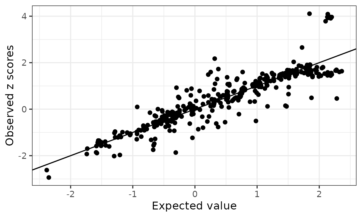

The default rule labels possible allele switches when logLR > 2 and abs(z) > 2.

outlier <- which(kr$conditional_dist$logLR > 2 &
                 abs(kr$conditional_dist$z) > 2)
length(outlier)
# [1] 0

For this example, the kriging diagnostic identifies 0 isolated allele switch outliers. This illustrates that kriging, designed for checking allele flips, does not work on this example which is not of that type of artifacts. It is not designed to model the broader finite LD reference error and mismatch between the LD reference panel and the target GWAS population that can affect an entire region.

Finite LD reference panel correction

The LD matrix here was computed from an LD reference panel of about 500 individuals. Setting R_finite = 500 tells susie_rss to account for this finite LD reference panel uncertainty in each SER update.

fit_B500 <- susie_rss(bhat = bhat, shat = shat,
                      R = R, n = n,
                      R_finite = 500)
# HINT: Setting max_iter = 50 for the SuSiE RSS model because slow convergence is often a sign of unstable summary-statistics fitting. To disable this message, explicitly set max_iter = 50 or another value in the susie_rss() call.
# HINT: Switching to PIP-based convergence: R uncertainty inflation modifies per-variant SER likelihoods, which prevents a consistent model-level ELBO.
# WARNING: IBSS algorithm did not converge in 50 iterations!
# Warning: IBSS algorithm did not converge in 50 iterations!
# WARNING: Possible summary statistics and R reference mismatch detected. Fine-mapping results may be unreliable; inspect fit$R_finite_diagnostics for details.
# Warning: Possible summary statistics and R reference mismatch detected.
# Fine-mapping results may be unreliable; inspect fit$R_finite_diagnostics for
# details.
count_cs(fit_B500)
# [1] 4

susie_plot(fit_B500, y = "PIP", add_legend = TRUE,
           main = "R_finite = 500")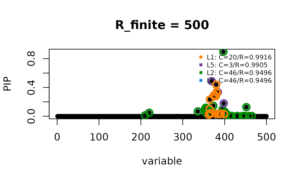

vapply(fit_B500$sets$cs, length, integer(1))
# L1 L5 L2 L7 
# 20  3 46 46
fit_B500$sets$purity
#    min.abs.corr mean.abs.corr median.abs.corr
# L1    0.9916071     0.9987394       0.9994052
# L5    0.9904815     0.9923051       0.9917869
# L2    0.9496351     0.9786389       0.9783094
# L7    0.9496351     0.9786389       0.9783094
cs_corr_B500 <- get_cs_correlation(fit_B500, Xcorr = R)
round(cs_corr_B500, 3)
#        L1     L5    L2    L7
# L1  1.000 -0.076 0.978 0.978
# L5 -0.076  1.000 0.120 0.120
# L2  0.978  0.120 1.000 1.000
# L7  0.978  0.120 1.000 1.000

In this subset of 500 variants, the finite LD reference correction reduces the result from 5 credible sets to 4. In the original larger region, using the same correction reduced the ordinary susie_rss result from 29 credible sets to 3. The credible sets also become less artificially sharp. Their sizes change from 2, 9, 9, 11 and 9 in the ordinary fit to 20, 3, 46 and 46, and the lowest purity drops from 0.9831 to 0.9496. The CS correlations are less uniformly extreme, but some remain high: one pair is still 1.000 and another is 0.978. Thus R_finite = 500 helps, but it does not fully resolve the mismatch pattern.

Empirical Bayes mismatch correction

Finite LD reference uncertainty only accounts for the fact that the LD matrix was estimated from a finite panel. It does not account for systematic mismatch due to drift between the LD reference population and the GWAS population. The option R_mismatch = "eb" estimates an additional variance component shared across the region from the fitted residuals.

fit_B500_eb <- susie_rss(bhat = bhat, shat = shat,
                         R = R, n = n,
                         R_finite = 500, R_mismatch = "eb")
# HINT: Setting max_iter = 50 for the SuSiE RSS model because slow convergence is often a sign of unstable summary-statistics fitting. To disable this message, explicitly set max_iter = 50 or another value in the susie_rss() call.
# HINT: Switching to PIP-based convergence: R uncertainty inflation modifies per-variant SER likelihoods, which prevents a consistent model-level ELBO.
# WARNING: Possible summary statistics and R reference mismatch detected. Fine-mapping results may be unreliable; inspect fit$R_finite_diagnostics for details. A one-effect diagnostic is available at fit$R_finite_diagnostics$ser_model; it is a one-effect credible-set model as in Maller et al. 2012, and its alpha row is the PIP.
# Warning: Possible summary statistics and R reference mismatch detected.
# Fine-mapping results may be unreliable; inspect fit$R_finite_diagnostics for
# details. A one-effect diagnostic is available at
# fit$R_finite_diagnostics$ser_model; it is a one-effect credible-set model as in
# Maller et al. 2012, and its alpha row is the PIP.
count_cs(fit_B500_eb)
# [1] 1

susie_plot(fit_B500_eb, y = "PIP", add_legend = TRUE,
           main = "R_finite = 500, R_mismatch = eb")

Here, adding R_mismatch = "eb" reduces the result to 1 credible set and the fit converges.

One can also run the mismatch model without specifying a finite LD reference panel size. This treats the continuous mismatch variance as the only LD uncertainty component.

fit_Binf_eb <- susie_rss(bhat = bhat, shat = shat,
                         R = R, n = n,
                         R_mismatch = "eb")
# HINT: Setting max_iter = 50 for the SuSiE RSS model because slow convergence is often a sign of unstable summary-statistics fitting. To disable this message, explicitly set max_iter = 50 or another value in the susie_rss() call.
# HINT: Switching to PIP-based convergence: R uncertainty inflation modifies per-variant SER likelihoods, which prevents a consistent model-level ELBO.
# WARNING: Possible summary statistics and R reference mismatch detected. Fine-mapping results may be unreliable; inspect fit$R_finite_diagnostics for details. A one-effect diagnostic is available at fit$R_finite_diagnostics$ser_model; it is a one-effect credible-set model as in Maller et al. 2012, and its alpha row is the PIP.
# Warning: Possible summary statistics and R reference mismatch detected.
# Fine-mapping results may be unreliable; inspect fit$R_finite_diagnostics for
# details. A one-effect diagnostic is available at
# fit$R_finite_diagnostics$ser_model; it is a one-effect credible-set model as in
# Maller et al. 2012, and its alpha row is the PIP.
count_cs(fit_Binf_eb)
# [1] 1

susie_plot(fit_Binf_eb, y = "PIP", add_legend = TRUE,
           main = "R_mismatch = eb")

This fit also reports 1 credible set and converges quickly.

vapply(fit_B500_eb$sets$cs, length, integer(1))
# L1 
# 34
fit_B500_eb$sets$purity
#    min.abs.corr mean.abs.corr median.abs.corr
# L1    0.8609486     0.9801885       0.9796367
max(fit_B500_eb$pip)
# [1] 0.1141644

In this subset, the two EB mismatch fits report the same 95% credible set. It contains 34 variants, has minimum purity 0.8609, and has coverage 0.9543; the largest PIP is 0.1142. Compared with the earlier fits, the EB adjustment keeps one signal but represents it as a broad credible set rather than several small, highly correlated credible sets. This is more consistent with the weak marginal association in this region.

In practice we recommend setting both R_finite and R_mismatch unless your reference LD is based on large samples such as current UK Biobank (300,000 to 500,000) in which case setting e.g. R_finite = 300000 will have no practical impact to the results.

Diagnostic metrics

The warnings above should not be ignored. Even after the EB adjustment, susie_rss reports diagnostic warnings, indicating that the fine mapping result remain uncertain. The fit object returns several diagnostic metrics to summarize this uncertainty.

fits <- list(susie_rss = fit_rss,
             R_finite_500 = fit_B500,
             R_finite_500_eb = fit_B500_eb,
             R_mismatch_eb = fit_Binf_eb)
knitr::kable(fit_table(fits), digits = 3)

	method	n_cs	niter	converged	Q_art	R_sensitivity_flag	R_reliability_flag
susie_rss	susie_rss	5	50	FALSE	NA	NA	NA
R_finite_500	R_finite_500	4	50	FALSE	NA	TRUE	TRUE
R_finite_500_eb	R_finite_500_eb	1	2	TRUE	0.12	FALSE	TRUE
R_mismatch_eb	R_mismatch_eb	1	2	TRUE	0.12	FALSE	TRUE

There are two relevant reliability diagnostics. Q_art measures whether the final residual points into directions where the supplied LD matrix has little support. R_sensitivity_flag measures whether reported credible sets depend strongly on the LD uncertainty penalty. If either diagnostic is triggered, R_reliability_flag is TRUE, and the fit should be interpreted cautiously.

In this subset, R_finite = 500 is flagged by the credible set sensitivity diagnostic. The two EB mismatch fits are flagged by the residual space diagnostic, even though they report only one credible set. This is why the warning points users to fit$R_finite_diagnostics rather than treating the corrected fit as automatically reliable.

Diagnostic with one effect

When the reliability flag is raised, the fit object provides a diagnostic model using single-effect regression (SER):

ser <- fit_Binf_eb$R_finite_diagnostics$ser_model
names(ser)
#  [1] "alpha"        "mu"           "mu2"          "lbf"          "lbf_variable"
#  [6] "V"            "KL"           "sigma2"       "pi"           "null_index"  
# [11] "niter"        "converged"    "pip"          "sets"

This is a credible set model with one effect as in Maller et al. (2012). For this model, the single row of alpha is the PIP.

identical(as.numeric(ser$alpha[1, ]), as.numeric(ser$pip))
# [1] TRUE
count_cs(ser)
# [1] 1
vapply(ser$sets$cs, length, integer(1))
# L1 
# 34
ser$sets$purity
#    min.abs.corr mean.abs.corr median.abs.corr
# L1    0.8609486     0.9801885       0.9796367
max(ser$pip)
# [1] 0.1141644
identical(ser$sets$cs, fit_Binf_eb$sets$cs)
# [1] TRUE
isTRUE(all.equal(as.numeric(ser$pip), as.numeric(fit_Binf_eb$pip)))
# [1] TRUE

susie_plot(ser, y = "PIP", add_legend = TRUE,
           main = "diagnostic with one effect")

In this example, the one-effect diagnostic gives the same result as the EB mismatch fit above: one 34-variant credible set, minimum purity 0.8609, and maximum PIP 0.1142. This exact match is merely a coincidence, not a general property of the method. When an EB mismatch fit produces a reliability warning, compare the EB result with this one-effect diagnostic rather than treating the EB fit as automatically reliable.

Summary

For routine analyses with GWAS summary statistics and an external LD reference panel:

First run basic allele and variant alignment quality control and checks. The kriging diagnostic can be useful for such obvious, localized allele coding artifacts.
Fit ordinary susie_rss and look for signs of instability, such as nonconvergence, multiple highly correlated credible sets, or many small credible sets in a weak association region.
Use R_finite when the LD matrix was estimated from a finite LD reference panel; add R_mismatch = "eb" when broader LD mismatch remains after accounting for finite reference uncertainty.
Inspect fit$R_finite_diagnostics, including Q_art, R_sensitivity_flag, and R_reliability_flag.
If a reliability warning is raised, compare the EB result with the SER diagnostic model, and interpret the fine-mapping result conservatively with the SER model as a safer fall-back.

Caution: allele coding artifacts are outside this model

The old RSS vignette example is based on the out-of-sample LD reference example from Zou et al. (2022). Because its LD matrix was computed from a finite reference panel of 500 individuals, it is appropriate to set R_finite = 500 when using the new diagnostics. This setting can raise a reliability warning, but that warning is not an allele flip correction and it does not replace allele alignment QC.

fit_toy_bad_B500_eb <- susie_rss(zflip, Rtoy, n = ntoy,
                                 R_finite = 500,
                                 R_mismatch = "eb",
                                 track_fit = TRUE)
d_toy <- fit_toy_bad_B500_eb$R_finite_diagnostics

knitr::kable(data.frame(
  n_cs = count_cs(fit_toy_bad_B500_eb),
  flipped_variant_pip =
    unname(fit_toy_bad_B500_eb$pip[SummaryConsistency$flip_id]),
  Q_art = d_toy$Q_art,
  residual_artifact_flag = d_toy$artifact_flag,
  CS_sensitivity_flag = d_toy$R_sensitivity_flag,
  overall_reliability_flag = d_toy$R_reliability_flag
), digits = 3, row.names = FALSE)

n_cs	flipped_variant_pip	Q_art	residual_artifact_flag	CS_sensitivity_flag	overall_reliability_flag
2	1	0.012	FALSE	TRUE	TRUE

susie_plot(fit_toy_bad_B500_eb, y = "PIP", b = btoy, add_legend = TRUE,
           main = "allele artifact with R_finite = 500, R_mismatch = eb")
points(SummaryConsistency$flip_id,
       fit_toy_bad_B500_eb$pip[SummaryConsistency$flip_id],
       col = 7, pch = 16)

This fit still reports 2 credible sets, and the flipped variant still has PIP close to 1. The residual artifact diagnostic does not flag this fit: Q_art is small and residual_artifact_flag is FALSE. However, the CS-level sensitivity diagnostic is TRUE, so the overall reliability flag is also TRUE. The warning therefore comes from CS sensitivity, not from Q_art.

This behavior is expected. The model in this vignette is designed for finite reference error and population drift in the LD matrix. It does not include an allele flip parameter, and it does not try to decide whether an individual z-score should have its sign reversed. That is deliberate: allele alignment is a data-processing problem that should be handled before fitting the LD mismatch model.

The reason is visible from the z-scores. Given the true signal and the LD matrix, the flipped variant should have a positive marginal association. Instead its observed z-score has the opposite sign.

flip_expected <- Rtoy[SummaryConsistency$flip_id,
                      SummaryConsistency$signal_id] *
                 zflip[SummaryConsistency$signal_id]
knitr::kable(data.frame(
  flipped_variant_z = zflip[SummaryConsistency$flip_id],
  LD_implied_z_from_signal = flip_expected,
  residual_after_signal = zflip[SummaryConsistency$flip_id] - flip_expected
), digits = 3)

flipped_variant_z	LD_implied_z_from_signal	residual_after_signal
-2.957	2.403	-5.36

This is a deterministic sign error at one variant, not the stochastic LD uncertainty modeled by R_finite or R_mismatch = "eb".

The compact track history can then be used to follow this specific artifact. We do not need to inspect the full object. For this toy example, the relevant rows are the single effects whose top variable is either the true signal or the known flipped variant. After the first IBSS iteration, one effect is already assigned almost entirely to the flipped variant.

track_toy <- fit_toy_bad_B500_eb$trace
track_effect <- subset(track_toy$effect,
                       iteration %in% 1:3 &
                       top_variable %in% c(SummaryConsistency$signal_id,
                                           SummaryConsistency$flip_id))
track_story <- data.frame(
  iteration = track_effect$iteration,
  effect = track_effect$effect,
  variant = paste0(track_effect$top_variable_name, " (", ifelse(
    track_effect$top_variable == SummaryConsistency$signal_id,
    "true signal",
    "flipped variant"
  ), ")"),
  alpha_at_variant = track_effect$top_alpha,
  max_variable_lbf = track_effect$top_lbf,
  single_effect_lbf = track_effect$effect_lbf
)

knitr::kable(track_story,
             digits = 3)

iteration	effect	variant	alpha_at_variant	max_variable_lbf	single_effect_lbf
1	1	rs62111707_T (true signal)	0.466	89.641	85.106
1	2	rs7257375_A (flipped variant)	0.982	8.412	3.132
2	1	rs62111707_T (true signal)	0.401	97.121	92.736
2	2	rs7257375_A (flipped variant)	0.999	10.675	5.378
3	1	rs62111707_T (true signal)	0.391	98.721	94.363
3	2	rs7257375_A (flipped variant)	1.000	12.080	6.782

Because this is a toy example, we know which variant is the true signal and which variant was deliberately flipped. The track table itself only shows the fitted single effect summaries: one effect is already highly concentrated on the flipped variant after the first iteration.

The CS-level diagnostic also shows why this happens. The fitted log BF and the log BF attenuation are different quantities: the former describes the fitted signal strength, whereas the latter measures how much that signal depends on uncertain LD.

cs_story <- track_toy$cs_sensitivity
final_effect <- track_toy$effect[
  track_toy$effect$iteration == max(track_toy$effect$iteration),
  c("effect", "top_lbf")
]
cs_story <- merge(cs_story, final_effect, by = "effect",
                  all.x = TRUE, sort = FALSE)
cs_story <- cs_story[cs_story$is_sensitive,
                     c("cs", "effect", "cs_size", "top_lbf",
                       "cs_max_bf_attenuation", "threshold",
                       "cs_sensitivity_label",
                       "top_sensitive_variable_name")]
names(cs_story) <- c("cs", "effect", "cs_size", "max_log_BF",
                     "log_BF_attenuation", "threshold", "sensitivity",
                     "sensitive_variant")
knitr::kable(cs_story,
             digits = 3)

cs	effect	cs_size	max_log_BF	log_BF_attenuation	threshold	sensitivity	sensitive_variant
L2	2	1	13.796	7.339	2.996	highly_sensitive	rs7257375_A
L1	1	5	99.495	7.230	2.996	highly_sensitive	rs62111707_T

For both credible sets, the attenuation is above the threshold log(20) = 3.0, so both are labeled highly_sensitive. This is why CS_sensitivity_flag is TRUE, and why the overall reliability flag is TRUE, even though Q_art = 0.012 and the residual artifact flag is FALSE.

Thus, an allele flip can create a convincing sparse effect before the LD mismatch model has anything useful to adjust. In this example, R_finite = 500 still raises a reliability warning through CS-level sensitivity, but that warning should be interpreted as a cue to inspect alignment, not as an automatic correction of the allele coding problem. In practice this warning is not guaranteed: for example, fitting this same toy example with R_mismatch = "eb" but without R_finite = 500 does not raise the reliability warning.

Session information

sessionInfo()
# R version 4.4.3 (2025-02-28)
# Platform: x86_64-conda-linux-gnu
# Running under: Ubuntu 24.04.4 LTS
# 
# Matrix products: default
# BLAS/LAPACK: /home/runner/work/susieR/susieR/.pixi/envs/r44/lib/libopenblasp-r0.3.33.so;  LAPACK version 3.12.0
# 
# locale:
#  [1] LC_CTYPE=C.UTF-8       LC_NUMERIC=C           LC_TIME=C.UTF-8       
#  [4] LC_COLLATE=C.UTF-8     LC_MONETARY=C.UTF-8    LC_MESSAGES=C.UTF-8   
#  [7] LC_PAPER=C.UTF-8       LC_NAME=C              LC_ADDRESS=C          
# [10] LC_TELEPHONE=C         LC_MEASUREMENT=C.UTF-8 LC_IDENTIFICATION=C   
# 
# time zone: Etc/UTC
# tzcode source: system (glibc)
# 
# attached base packages:
# [1] stats     graphics  grDevices utils     datasets  methods   base     
# 
# other attached packages:
# [1] susieR_0.16.1
# 
# loaded via a namespace (and not attached):
#  [1] Matrix_1.7-5          gtable_0.3.6          jsonlite_2.0.0       
#  [4] compiler_4.4.3        crayon_1.5.3          Rcpp_1.1.1-1.1       
#  [7] jquerylib_0.1.4       systemfonts_1.3.2     scales_1.4.0         
# [10] textshaping_1.0.5     yaml_2.3.12           fastmap_1.2.0        
# [13] lattice_0.22-9        plyr_1.8.9            ggplot2_4.0.3        
# [16] R6_2.6.1              labeling_0.4.3        mixsqp_0.3-54        
# [19] knitr_1.51            htmlwidgets_1.6.4     desc_1.4.3           
# [22] zigg_0.0.2            bslib_0.10.0          RColorBrewer_1.1-3   
# [25] rlang_1.2.0           reshape_0.8.10        cachem_1.1.0         
# [28] xfun_0.57             fs_2.1.0              sass_0.4.10          
# [31] S7_0.2.2              RcppParallel_5.1.11-2 otel_0.2.0           
# [34] cli_3.6.6             withr_3.0.2           pkgdown_2.2.0        
# [37] digest_0.6.39         grid_4.4.3            irlba_2.3.7          
# [40] lifecycle_1.0.5       vctrs_0.7.3           Rfast_2.1.5.2        
# [43] evaluate_1.0.5        glue_1.8.1            farver_2.1.2         
# [46] ragg_1.5.2            rmarkdown_2.31        matrixStats_1.5.0    
# [49] tools_4.4.3           htmltools_0.5.9

Reference

Maller JB, McVean G, Byrnes J, Vukcevic D, Palin K, Su Z, et al. Bayesian refinement of association signals for 14 loci in 3 common diseases. Nature Genetics 44, 1294-1301 (2012).

Gao Wang

2026-05-13