Fine-mapping with summary statistics
Yuxin Zou and Gao Wang
2026-05-01
Source:vignettes/finemapping_summary_statistics.Rmd
finemapping_summary_statistics.RmdThis vignette demonstrates how to use susieR with
“summary statistics” in the context of genetic fine-mapping. We use the
same simulated data as in fine mapping
vignette. The simulated data are expression levels of a gene (y) in N \approx
600 individuals. We want to identify with the genotype matrix
X_{N\times
P} (P=1001) the genetic
variables that causes changes in expression level. This data set is
shipped with susieR. It is simulated to have exactly three
non-zero effects.
The data-set
Notice that we’ve simulated two sets of Y as two simulation replicates. Here we’ll focus on the first data-set.
dim(Y)
# [1] 574   2
Here are the three true signals in the first data-set:
b <- true_coef[,1]
plot(b, pch=16, ylab='effect size')
which(b != 0)
# [1] 403 653 773
So the underlying causal variables are 403, 653 and 773.
Summary statistics from simple regression
Summary statistics of genetic association studies typically contain effect sizes (\hat{\beta} coefficient from regression) and p-values. These statisticscan be used to perform fine-mapping with given an additional input of correlation matrix between variables. The correlation matrix in genetics is typically referred to as an “LD matrix” (LD is short for linkage disequilibrium). One may use external reference panels to estimate it when this matrix cannot be obtained from samples directly. Importantly, the LD matrix has to be a matrix containing estimates of the correlation, r, and not r^2 or |r|. See also this vignette for how to check the consistency of the LD matrix with the summary statistics.
The univariate_regression function can be used to
compute summary statistics by fitting univariate simple regression
variable by variable. The results are \hat{\beta} and SE(\hat{\beta}) from which z-scores can be
derived. Alternatively, you can obtain z-scores from \hat{\beta} and p-values if you are provided
with those information. For example,
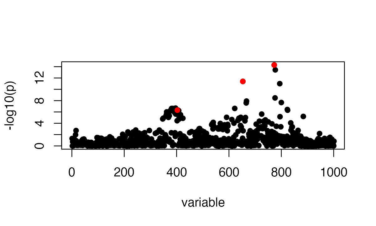
sumstats <- univariate_regression(X, Y[,1])
z_scores <- sumstats$betahat / sumstats$sebetahat
susie_plot(z_scores, y = "z", b=b)
For this example, the correlation matrix can be computed directly from data provided:
R <- cor(X)Fine-mapping with susieR using summary statistics
By default, SuSiE assumes at most 10 causal variables, with
L = 10, although we note that SuSiE is generally robust to
the choice of L.
Since the individual-level data is available for us here, we can
easily compute the “in-sample LD” matrix, as well as the variance of
y, which is 7.8424. (By “in-sample”, we
means the LD was computed from the exact same matrix X that
was used to obtain the other statistics.) When we fit SuSiE regression
with summary statistics, \hat{\beta},
SE(\hat{\beta}), R, n, and
var_y these are also the sufficient statistics. With an
in-sample LD, we can also estimate the residual variance using these
sufficient statistics. (Note that if the covariate effects are removed
from the genotypes in the univariate regression, it is recommended that
the “in-sample” LD matrix also be computed from the genotypes after the
covariate effects have been removed.)
fitted_rss1 <- susie_rss(bhat = sumstats$betahat, shat = sumstats$sebetahat, n = n, R = R, var_y = var(Y[,1]), L = 10,
                         estimate_residual_variance = TRUE)
# WARNING: For estimate_residual_variance = TRUE, please check that R is the "in-sample" R matrix; that is, the correlation matrix obtained using the exact same data matrix X that was used for the other summary statistics. Also note, when covariates are included in the univariate regressions that produced the summary statistics, also consider removing these effects from X before computing R.
Using summary, we can examine the posterior inclusion
probability (PIP) for each variable, and the 95% credible sets:
summary(fitted_rss1)$cs
#   cs cs_log10bf cs_avg_r2 cs_min_r2
# 1  2   4.034050 1.0000000 1.0000000
# 2  1   6.742404 0.9634847 0.9634847
# 3  3   3.461519 0.9224322 0.7545197
#                                                                                                                  variable
# 1                                                                                                                     653
# 2                                                                                                                 773,777
# 3 362,365,366,367,368,372,373,374,379,381,383,384,386,387,388,389,391,392,396,397,398,399,400,401,403,404,405,407,408,415
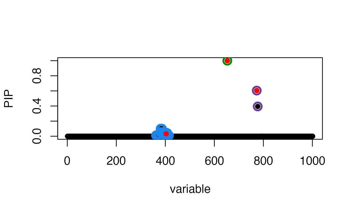
The three causal signals have been captured by the three CSs. Note the third CS contains many variables, including the true causal variable 403.
We can also plot the posterior inclusion probabilities (PIPs):
susie_plot(fitted_rss1, y="PIP", b=b)
The true causal variables are shown in red. The 95% CSs are shown by three different colours (green, purple, blue).
Note this result is exactly the same as running
susie on the original individual-level data:
fitted = susie(X, Y[,1], L = 10)
all.equal(fitted$pip, fitted_rss1$pip)
# [1] TRUE
all.equal(coef(fitted)[-1], coef(fitted_rss1)[-1])
# [1] TRUE
If, on the other hand, the variance of y is unknown, we fit can SuSiE regression with summary statistics, \hat{\beta}, SE(\hat{\beta}), R and n (or z-scores, R and n). The outputted effect estimates are now on the standardized X and y scale. Still, we can estimate the residual variance because we have the in-sample LD matrix:
fitted_rss2 = susie_rss(z = z_scores, R = R, n = n, L = 10,
                        estimate_residual_variance = TRUE)
# WARNING: For estimate_residual_variance = TRUE, please check that R is the "in-sample" R matrix; that is, the correlation matrix obtained using the exact same data matrix X that was used for the other summary statistics. Also note, when covariates are included in the univariate regressions that produced the summary statistics, also consider removing these effects from X before computing R.
The result is same as if we had run susie on the
individual-level data, but the output effect estimates are on different
scale:
all.equal(fitted$pip, fitted_rss2$pip)
# [1] TRUE
plot(coef(fitted)[-1], coef(fitted_rss2)[-1], xlab = 'effects from SuSiE', ylab = 'effects from SuSiE-RSS', xlim=c(-1,1), ylim=c(-0.3,0.3))
Specifically, without the variance of y, these estimates are same as if we had applied SuSiE to a standardized X and y; that is, as if y and the columns of X had been normalized so that y and each column of X had a standard deviation of 1.
Fine-mapping with susieR using LD matrix from reference
panel
When the original genotypes are not available, one may use a separate reference panel to estimate the LD matrix.
To illustrate this, we randomly generated 500 samples from N(0,R) and treated them as reference panel
genotype matrix X_ref.
We fit the SuSiE regression using out-of sample LD matrix. The residual variance is fixed at 1 because estimating residual variance sometimes produces very inaccurate estimates with out-of-sample LD matrix. The output effect estimates are on the standardized X and y scale.
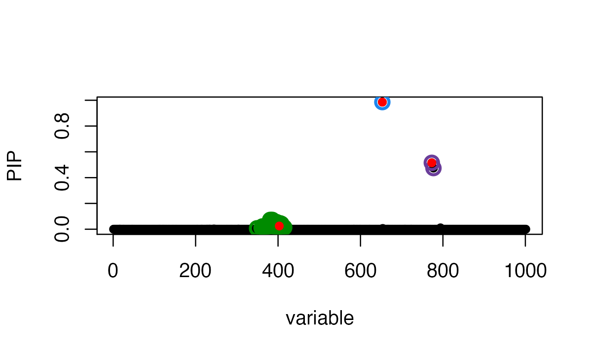
fitted_rss3 <- susie_rss(z_scores, R_ref, n=n, L = 10)
susie_plot(fitted_rss3, y="PIP", b=b)
In this particular example, the SuSiE result with out-of-sample LD is very similar to using the in-sample LD matrix because the LD matrices are quite similar.

In some rare cases, the sample size n is unknown. When the sample size is not
provided as input to susie_rss, this is in effect assuming
the sample size is infinity and all the effects are small, and the
estimated PVE for each variant will be close to zero. The outputted
effect estimates are on the “noncentrality parameter” scale.
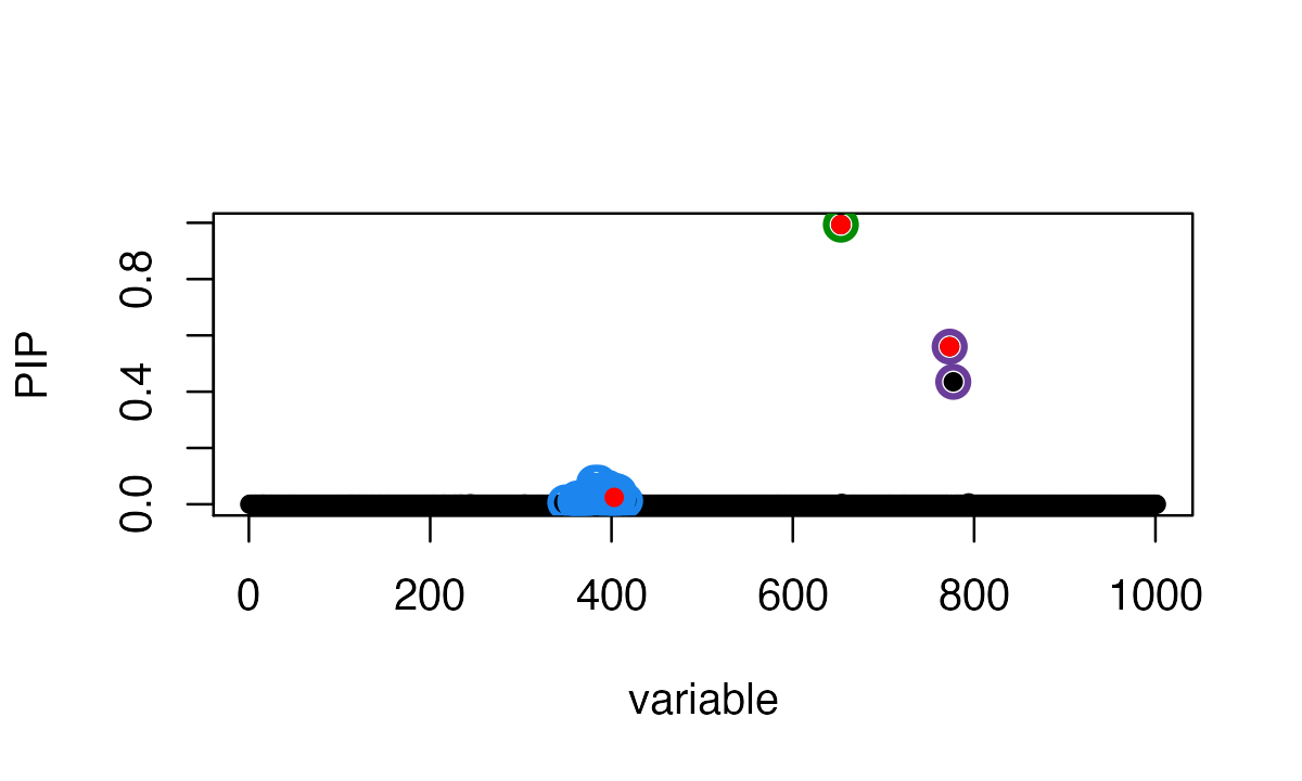
fitted_rss4 = susie_rss(z_scores, R_ref, L = 10)
# WARNING: Providing the sample size (n), or even a rough estimate of n, is highly recommended. Without n, the implicit assumption is n is large (Inf) and the effect sizes are small (close to zero).
susie_plot(fitted_rss4, y="PIP", b=b)
Session information
Here are some details about the computing environment, including the versions of R, and the R packages, used to generate these results.
sessionInfo()
# R version 4.4.3 (2025-02-28)
# Platform: x86_64-conda-linux-gnu
# Running under: Ubuntu 24.04.4 LTS
#
# Matrix products: default
# BLAS/LAPACK: /home/runner/work/susieR/susieR/.pixi/envs/r44/lib/libopenblasp-r0.3.32.so;  LAPACK version 3.12.0
#
# locale:
#  [1] LC_CTYPE=C.UTF-8       LC_NUMERIC=C           LC_TIME=C.UTF-8
#  [4] LC_COLLATE=C.UTF-8     LC_MONETARY=C.UTF-8    LC_MESSAGES=C.UTF-8
#  [7] LC_PAPER=C.UTF-8       LC_NAME=C              LC_ADDRESS=C
# [10] LC_TELEPHONE=C         LC_MEASUREMENT=C.UTF-8 LC_IDENTIFICATION=C
#
# time zone: Etc/UTC
# tzcode source: system (glibc)
#
# attached base packages:
# [1] stats     graphics  grDevices utils     datasets  methods   base
#
# other attached packages:
# [1] susieR_0.16.1
#
# loaded via a namespace (and not attached):
#  [1] Matrix_1.7-5          gtable_0.3.6          jsonlite_2.0.0
#  [4] compiler_4.4.3        crayon_1.5.3          Rcpp_1.1.1-1.1
#  [7] jquerylib_0.1.4       systemfonts_1.3.2     scales_1.4.0
# [10] textshaping_1.0.5     yaml_2.3.12           fastmap_1.2.0
# [13] lattice_0.22-9        plyr_1.8.9            ggplot2_4.0.3
# [16] R6_2.6.1              mixsqp_0.3-54         knitr_1.51
# [19] htmlwidgets_1.6.4     desc_1.4.3            zigg_0.0.2
# [22] bslib_0.10.0          RColorBrewer_1.1-3    rlang_1.2.0
# [25] reshape_0.8.10        cachem_1.1.0          xfun_0.57
# [28] fs_2.1.0              sass_0.4.10           S7_0.2.2
# [31] RcppParallel_5.1.11-2 otel_0.2.0            cli_3.6.6
# [34] pkgdown_2.2.0         digest_0.6.39         grid_4.4.3
# [37] irlba_2.3.7           lifecycle_1.0.5       vctrs_0.7.3
# [40] Rfast_2.1.5.2         evaluate_1.0.5        glue_1.8.1
# [43] farver_2.1.2          ragg_1.5.2            rmarkdown_2.31
# [46] matrixStats_1.5.0     tools_4.4.3           htmltools_0.5.9