susie_plot produces a per-variable summary of
the SuSiE credible sets. susie_plot_iteration produces a
diagnostic plot for the susie model fitting. For
susie_plot_iteration, several plots will be created if
track_fit = TRUE when calling susie.
Usage
susie_plot(
  model,
  y,
  add_bar = FALSE,
  pos = NULL,
  b = NULL,
  max_cs = 400,
  add_legend = NULL,
  ...
)

susie_plot_iteration(model, L, file_prefix, pos = NULL)
Arguments
- model
A SuSiE fit, typically an output from
susieor one of its variants. Forsuse_plot, the susie fit must havemodel$z,model$PIP, and may includemodel$sets.modelmay also be a vector of z-scores or PIPs. Forsusie_plot_iteration,modelmust be either a SuSiE fit or itssusie_trackobject frommodel$trace.- y
A string indicating what to plot: either
"z_original"for z-scores,"z"for z-score derived p-values on (base-10) log-scale,"PIP"for posterior inclusion probabilities,"log10PIP"for posterior inclusion probabiliities on the (base-10) log-scale. For any other setting, the data are plotted as is.- add_bar
If
add_bar = TRUE, add horizontal bar to signals in credible interval.- pos
Indices of variables to plot. If
pos = NULLall variables are plotted.- b
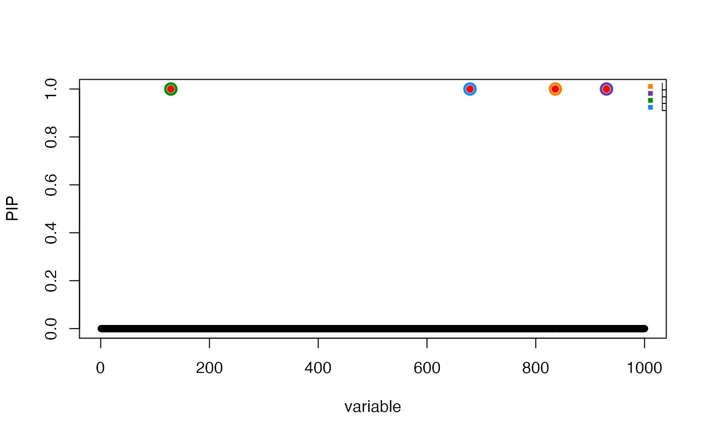
For simulated data, set
b = TRUEto highlight "true" effects (highlights in red).- max_cs
The largest credible set to display, either based on purity (set
max_csbetween 0 and 1), or based on size (setmax_cs > 1).- add_legend
If
add_legend = TRUE, add a legend to annotate the size and purity of each CS discovered. It can also be specified as location where legends should be added, e.g.,add_legend = "bottomright"(default location is"topright").- ...
Additional arguments passed to
plot.- L
An integer specifying the number of single-effect rows to plot.
- file_prefix
Prefix to path of output plot file. If not specified, the plot, or plots, will be saved to a temporary directory generated using
tempdir.
Examples
set.seed(1)
n <- 1000
p <- 1000
beta <- rep(0, p)
beta[sample(1:1000, 4)] <- 1
X <- matrix(rnorm(n * p), nrow = n, ncol = p)
X <- scale(X, center = TRUE, scale = TRUE)
y <- drop(X %*% beta + rnorm(n))
res <- susie(X, y, L = 10)
susie_plot(res, "PIP")
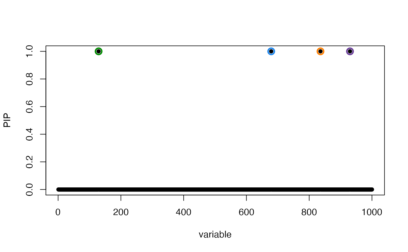 susie_plot(res, "PIP", add_bar = TRUE)
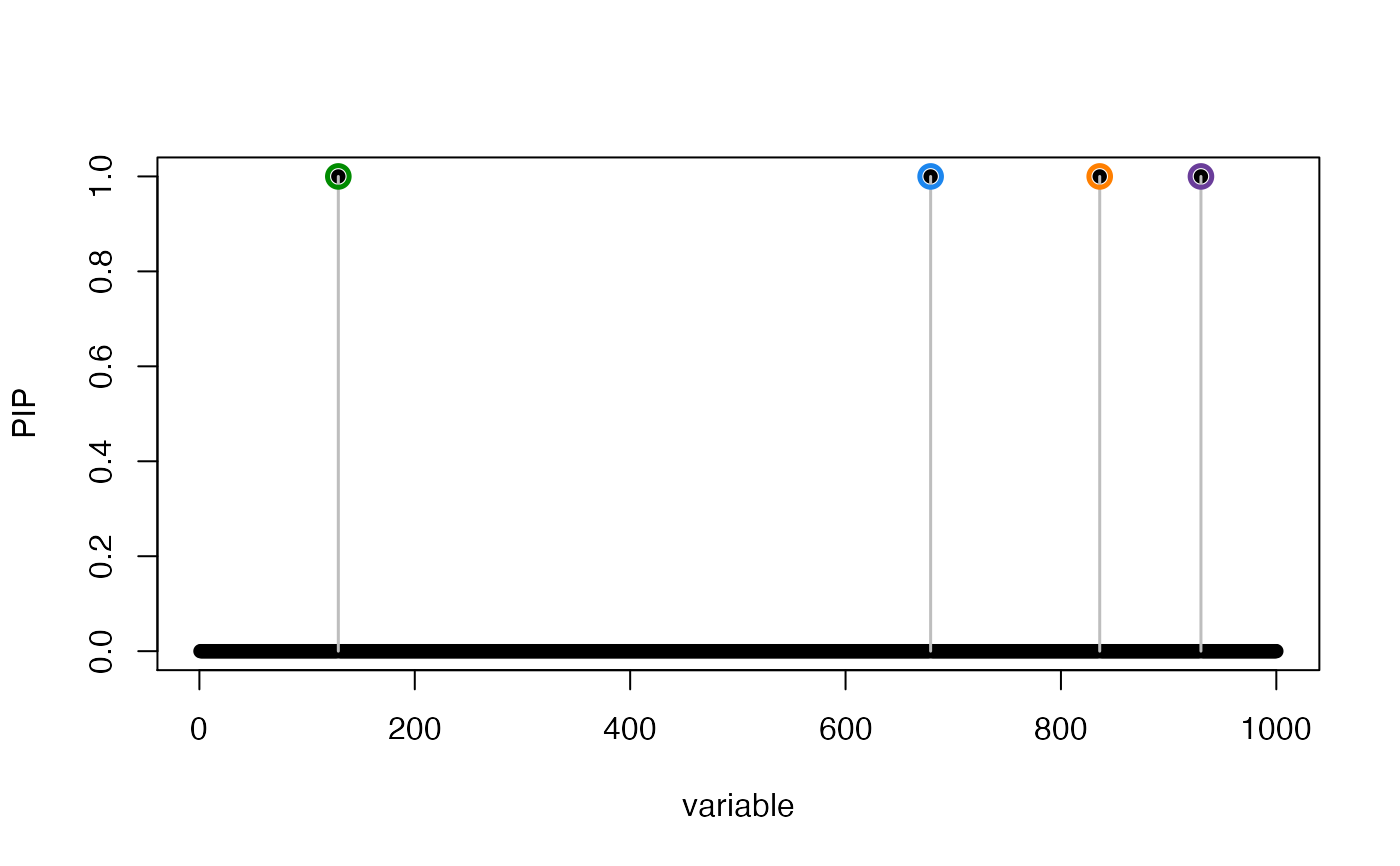 susie_plot(res, "PIP", add_legend = TRUE)
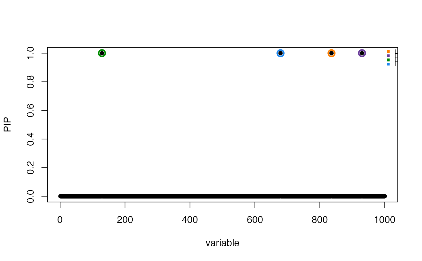 susie_plot(res, "PIP", pos = 1:500, add_legend = TRUE)
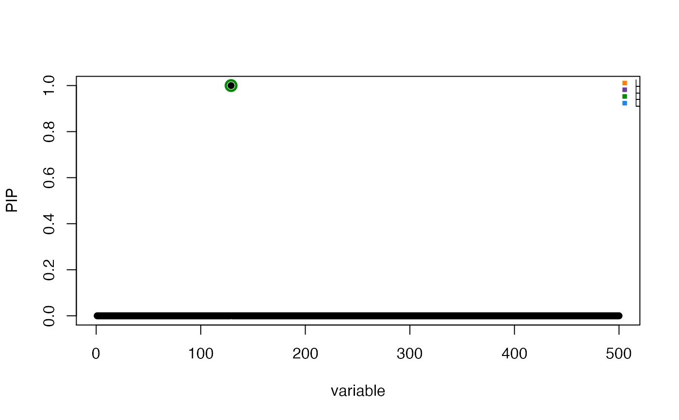 # Plot selected regions with adjusted x-axis position label
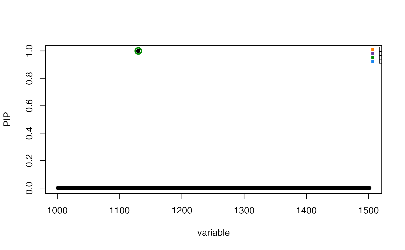
res$genomic_position <- 1000 + (1:length(res$pip))
susie_plot(res, "PIP",
add_legend = TRUE,
pos = list(attr = "genomic_position", start = 1000, end = 1500)
)
 # True effects are shown in red.
susie_plot(res, "PIP", b = beta, add_legend = TRUE)
 set.seed(1)
n <- 1000
p <- 1000
beta <- rep(0, p)
beta[sample(1:1000, 4)] <- 1
X <- matrix(rnorm(n * p), nrow = n, ncol = p)
X <- scale(X, center = TRUE, scale = TRUE)
y <- drop(X %*% beta + rnorm(n))
res <- susie(X, y, L = 10, track_fit = TRUE)
susie_plot_iteration(res, L = 10)
#> Creating GIF animation...
#> Warning: error in running command
#> Iterplot saved to /tmp/RtmptncQSC/susie_plot.gif