Diagnostic for fine-mapping with summary statistics
Yuxin Zou
2026-05-13
Source:vignettes/susierss_diagnostic.Rmd
susierss_diagnostic.RmdThis vignette demonstrates the use of the diagnostic plot for assessing consistency of the summary statistics and the reference LD matrix.
This vignette focuses on diagnosing inconsistencies such as allele coding artifacts. For model-based ways to account for finite or mismatched LD reference panels in fine mapping, see this vignette.
The susie_rss assumes the LD matrix accurately estimate
the correlations among SNPs from the original GWAS genotype data.
Typically, the LD matrix comes from some public database of genotypes in
a suitable reference population. The inaccurate LD information leads to
unreliable fine-mapping result.
The diagnostic for consistency between summary statistics and refenrence LD matrix is based on the RSS model under the null with regularized LD matrix. \hat{z} | R, \lambda \sim N(0, (1-\lambda)R + \lambda I), 0<\lambda<1 The parameter \lambda is estimated by maximum likelihood. A larger \lambda means a greater inconsistency between summary statistics and the LD matrix. The expected z score is computed for each SNP, E(\hat{z}_j | \hat{z}_{-j}), and plotted against the observed z scores.
LD information from the original genotype data
We demonstrate the diagnostic plot in a simple case, the LD matrix is estimated from the original genotype data. In this case, we expect the diagnostic plot to confirm that the LD matrix is consistent with the z scores.
We use the same simulated data as in fine mapping vignette.
data("N3finemapping")
n = nrow(N3finemapping$X)
b = N3finemapping$true_coef[,1]
sumstats <- univariate_regression(N3finemapping$X, N3finemapping$Y[,1])
z_scores <- sumstats$betahat / sumstats$sebetahat
Rin = cor(N3finemapping$X)
attr(Rin, "eigen") = eigen(Rin, symmetric = TRUE)
susie_plot(z_scores, y = "z", b=b)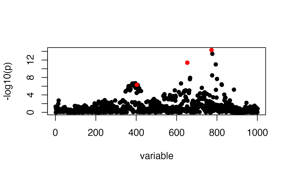
The estimated \lambda is
lambda = estimate_s_rss(z_scores, Rin, n=n)
lambda
# [1] 6.474096e-09
The plot for the observed z scores vs the expected z scores is
condz_in = kriging_rss(z_scores, Rin, n=n)
condz_in$plot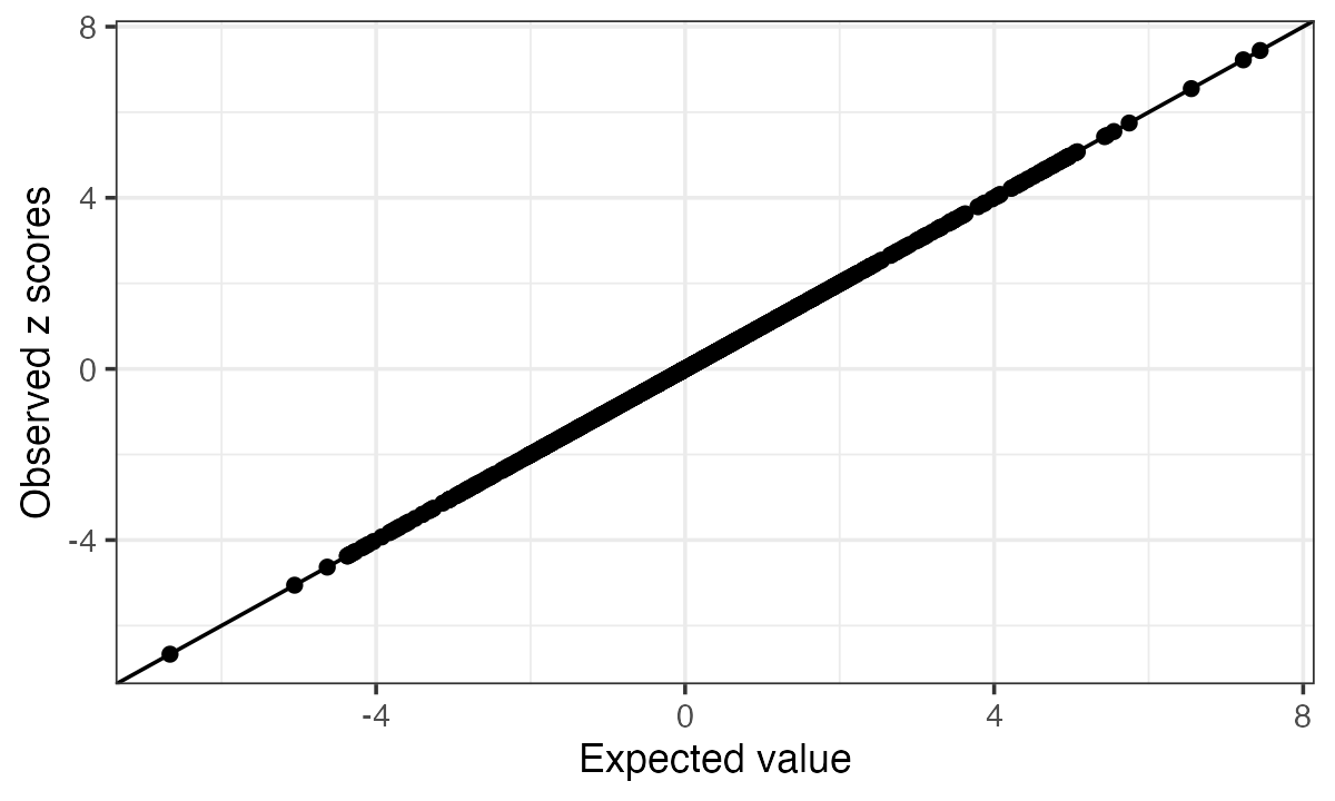
Summary of SuSiE Credible Sets:
fit <- susie_rss(z_scores, Rin, n=n, estimate_residual_variance = TRUE)
# HINT: Setting max_iter = 50 for the SuSiE RSS model because slow convergence is often a sign of unstable summary-statistics fitting. To disable this message, explicitly set max_iter = 50 or another value in the susie_rss() call.
# WARNING: estimate_residual_variance = TRUE is not recommended unless R is the "in-sample" R matrix; that is, the correlation matrix obtained using the exact same data matrix X that was used for the other summary statistics. If R is in-sample, set R_finite = FALSE to silence this warning. When covariates are included in the univariate regressions that produced the summary statistics, also consider removing these effects from X before computing R.
susie_plot(fit,y = "PIP", b=b)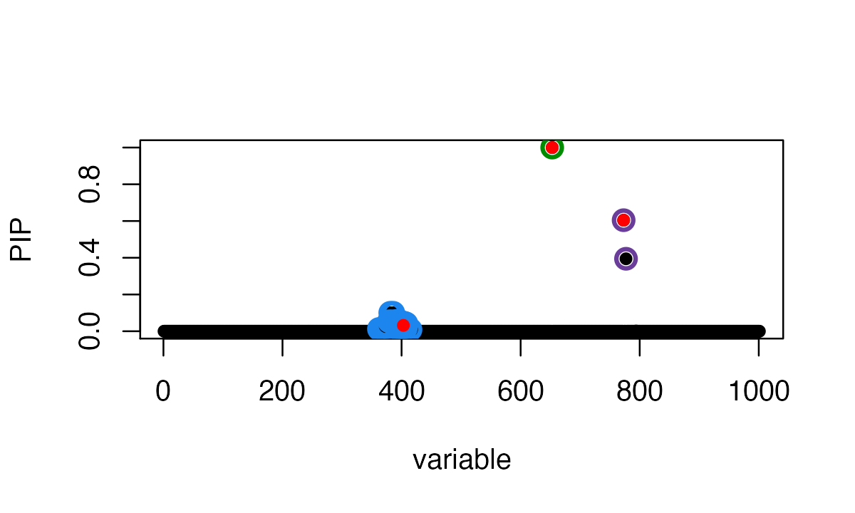
LD information from the reference panel
We use another simulated data where the LD matrix is estimated from a reference panel. In this example data set, there is one association signal in the simulated data (red point), and there is one SNP with mismatched reference and alternative allele between summary statistics and the reference panel (yellow point).
Note: In some versions of PLINK, these mismatches
can occur when PLINK
automatically flips the alleles to make the minor allele be the effect
allele, leading to different allele encodings in the z scores and LD
matrix. Adding the flag --keep-allele-order will disable
this behaviour in PLINK.
data_file <- tempfile(fileext = ".RData")
data_url <- paste0("https://raw.githubusercontent.com/stephenslab/susieR/",
                   "master/inst/datafiles/SummaryConsistency1k.RData")
curl_download(data_url,data_file)
load(data_file)
zflip = SummaryConsistency$z
ld = SummaryConsistency$ldref
n=10000
b = numeric(length(zflip))
b[SummaryConsistency$signal_id] = zflip[SummaryConsistency$signal_id]
plot(zflip, pch = 16, col = "#767676", main = "Marginal Associations",
     xlab="SNP", ylab = "z scores")
points(SummaryConsistency$signal_id, zflip[SummaryConsistency$signal_id], col=2, pch=16)
points(SummaryConsistency$flip_id, zflip[SummaryConsistency$flip_id], col=7, pch=16)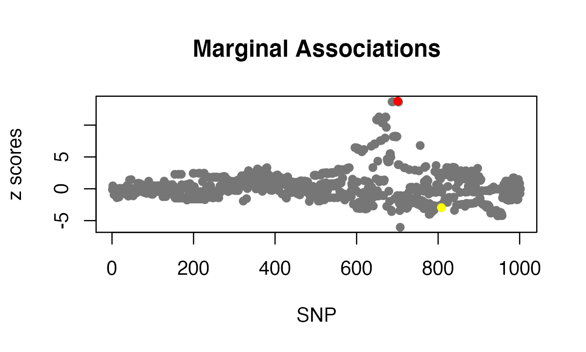
Using the data with misaligned allele, SuSiE-RSS identifies a true positive CS containing the true effect SNP; and a false positive CS that incorrectly contains the mismatched SNP.
fit = susie_rss(zflip, ld, n=n)
# HINT: Setting max_iter = 50 for the SuSiE RSS model because slow convergence is often a sign of unstable summary-statistics fitting. To disable this message, explicitly set max_iter = 50 or another value in the susie_rss() call.
susie_plot(fit, y='PIP', b=b)
points(SummaryConsistency$flip_id, fit$pip[SummaryConsistency$flip_id], col=7, pch=16)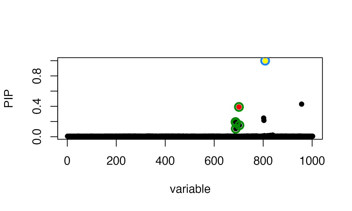
The estimated \lambda is
lambda = estimate_s_rss(zflip, ld, n=n)
lambda
# [1] 0.005005011
In the diagnostic plot, the mismatched SNP shows the largest difference between observed and expected z-scores, and therefore appears furthest away from the diagonal.
condz = kriging_rss(zflip, ld, n=n)
condz$plot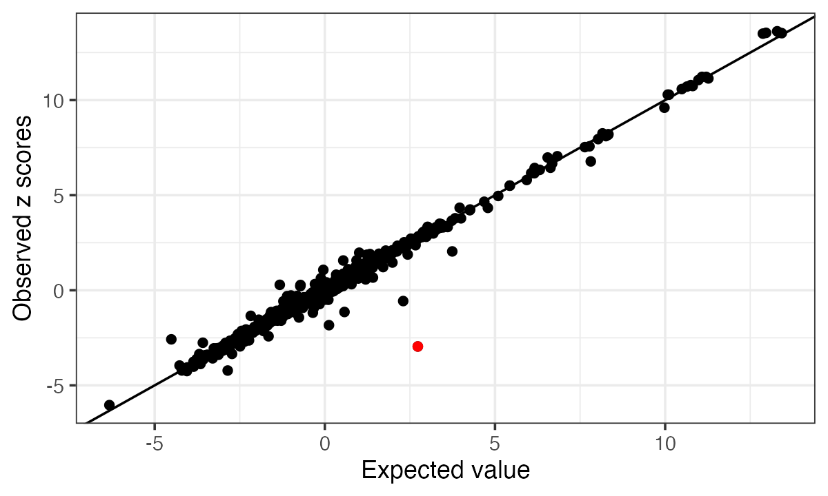
After fixing the allele encoding, SuSiE-RSS identifies a single true positive CS containing the true-effect SNP, and the formerly mismatched SNP is (correctly) not included in a CS.
z = zflip
z[SummaryConsistency$flip_id] = -z[SummaryConsistency$flip_id]
fit = susie_rss(z, ld, n=n)
# HINT: Setting max_iter = 50 for the SuSiE RSS model because slow convergence is often a sign of unstable summary-statistics fitting. To disable this message, explicitly set max_iter = 50 or another value in the susie_rss() call.
susie_plot(fit, y='PIP', b=b)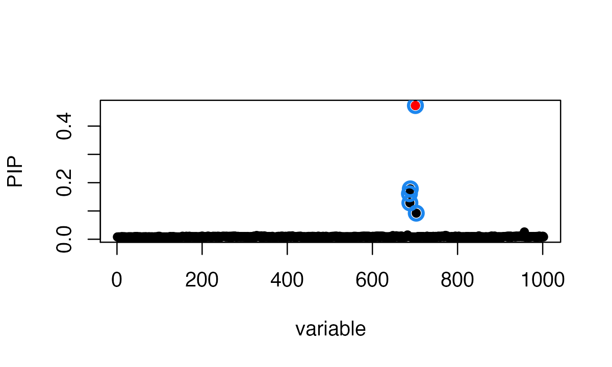
Session information
Here are some details about the computing environment, including the versions of R, and the R packages, used to generate these results.
sessionInfo()
# R version 4.4.3 (2025-02-28)
# Platform: x86_64-conda-linux-gnu
# Running under: Ubuntu 24.04.4 LTS
#
# Matrix products: default
# BLAS/LAPACK: /home/runner/work/susieR/susieR/.pixi/envs/r44/lib/libopenblasp-r0.3.33.so;  LAPACK version 3.12.0
#
# locale:
#  [1] LC_CTYPE=C.UTF-8       LC_NUMERIC=C           LC_TIME=C.UTF-8
#  [4] LC_COLLATE=C.UTF-8     LC_MONETARY=C.UTF-8    LC_MESSAGES=C.UTF-8
#  [7] LC_PAPER=C.UTF-8       LC_NAME=C              LC_ADDRESS=C
# [10] LC_TELEPHONE=C         LC_MEASUREMENT=C.UTF-8 LC_IDENTIFICATION=C
#
# time zone: Etc/UTC
# tzcode source: system (glibc)
#
# attached base packages:
# [1] stats     graphics  grDevices utils     datasets  methods   base
#
# other attached packages:
# [1] curl_7.1.0    susieR_0.16.1
#
# loaded via a namespace (and not attached):
#  [1] Matrix_1.7-5          gtable_0.3.6          jsonlite_2.0.0
#  [4] compiler_4.4.3        crayon_1.5.3          Rcpp_1.1.1-1.1
#  [7] jquerylib_0.1.4       systemfonts_1.3.2     scales_1.4.0
# [10] textshaping_1.0.5     yaml_2.3.12           fastmap_1.2.0
# [13] lattice_0.22-9        plyr_1.8.9            ggplot2_4.0.3
# [16] R6_2.6.1              labeling_0.4.3        mixsqp_0.3-54
# [19] knitr_1.51            htmlwidgets_1.6.4     desc_1.4.3
# [22] zigg_0.0.2            bslib_0.10.0          RColorBrewer_1.1-3
# [25] rlang_1.2.0           reshape_0.8.10        cachem_1.1.0
# [28] xfun_0.57             fs_2.1.0              sass_0.4.10
# [31] S7_0.2.2              RcppParallel_5.1.11-2 otel_0.2.0
# [34] cli_3.6.6             withr_3.0.2           pkgdown_2.2.0
# [37] digest_0.6.39         grid_4.4.3            irlba_2.3.7
# [40] lifecycle_1.0.5       vctrs_0.7.3           Rfast_2.1.5.2
# [43] evaluate_1.0.5        glue_1.8.1            farver_2.1.2
# [46] ragg_1.5.2            rmarkdown_2.31        matrixStats_1.5.0
# [49] tools_4.4.3           htmltools_0.5.9