Compute Distribution of z-scores of Variant j Given Other z-scores, and Detect Possible Allele Switch Issue

Under the null, the rss model with regularized LD matrix is \(z|R,s ~ N(0, (1-s)R + s I))\). We use a mixture of normals to model the conditional distribution of z_j given other z scores, \(z_j | z_{-j}, R, s ~ \sum_{k=1}^{K} \pi_k N(-\Omega_{j,-j} z_{-j}/\Omega_{jj}, \sigma_{k}^2/\Omega_{jj})\), \(\Omega = ((1-s)R + sI)^{-1}\), \(\sigma_1, ..., \sigma_k\) is a grid of fixed positive numbers. We estimate the mixture weights \(\pi\) We detect the possible allele switch issue using likelihood ratio for each variant.

Usage

kriging_rss(
  z,
  R,
  n,
  r_tol = 1e-08,
  s = estimate_s_rss(z, R, n, r_tol, method = "null-mle")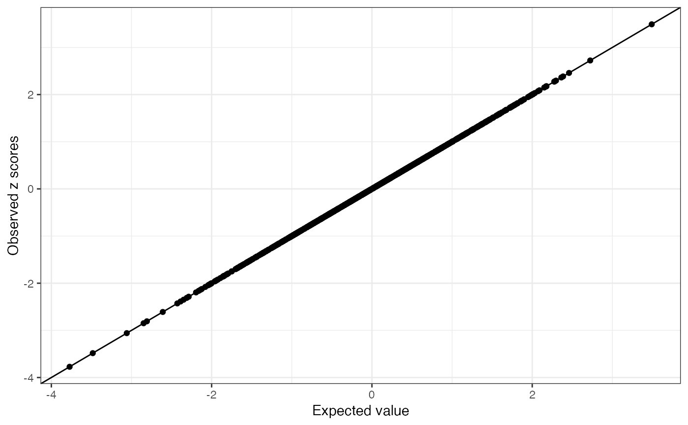
)

Arguments

z

A p-vector of z scores.

R

A p by p symmetric, positive semidefinite correlation matrix.

n

The sample size. (Optional, but highly recommended.)

r_tol

Tolerance level for eigenvalue check of positive semidefinite matrix of R.

s

an estimated s from estimate_s_rss

Value

a list containing a ggplot2 plot object and a table. The plot compares observed z score vs the expected value. The possible allele switched variants are labeled as red points (log LR > 2 and abs(z) > 2). The table summarizes the conditional distribution for each variant and the likelihood ratio test. The table has the following columns: the observed z scores, the conditional expectation, the conditional variance, the standardized differences between the observed z score and expected value, the log likelihood ratio statistics.

Examples

# See also the vignette, "Diagnostic for fine-mapping with summary
# statistics."
set.seed(1)
n <- 500
p <- 1000
beta <- rep(0, p)
beta[1:4] <- 0.01
X <- matrix(rnorm(n * p), nrow = n, ncol = p)
X <- scale(X, center = TRUE, scale = TRUE)
y <- drop(X %*% beta + rnorm(n))
ss <- univariate_regression(X, y)
R <- cor(X)
attr(R, "eigen") <- eigen(R, symmetric = TRUE)
zhat <- with(ss, betahat / sebetahat)
cond_dist <- kriging_rss(zhat, R, n = n)
cond_dist$plot