Interpreting and visualizing mvSuSiE results

This vignette demonstrates how to interpret the output of a fitted mvSuSiE model, including credible sets, posterior inclusion probabilities (PIPs), effect estimates, and local false sign rates (LFSR). We also show the built-in visualization functions.

library(mvsusieR)
library(ggplot2)
library(cowplot)
set.seed(1)

We use the built-in simdata data set, which contains realistic genotypes and simulated phenotypes for 20 traits with three causal SNPs.

data(simdata)
X <- simdata$raw$X
Y <- simdata$raw$Y
cat(sprintf("Data: %d samples, %d SNPs, %d traits\n",
            nrow(X), ncol(X), ncol(Y)))

prior <- create_mixture_prior(list(matrices = simdata$par$U,
                                   weights = simdata$par$w),
                              null_weight = 0)
fit <- mvsusie(X, Y, 
               prior_variance = prior,
               residual_variance = simdata$par$V)
# mvsusie: N=574, J=1001, R=20, L=10 [mem: 0.16 GB]
# Residual variance set, common_cov=TRUE [mem: 0.16 GB]
# Prior: K=19 mixture components [mem: 0.16 GB]
# Eigendecomposition cache: K=19, common_cov=TRUE [mem: 0.17 GB]
# Model initialized: J=1001, R=20, L=10, K=19 [mem: 0.17 GB]
# iter          ELBO       delta   sigma2      mem      V
#    1   -15961.8377           -   diag[0.845,1.08]   0.17 GB  [6.82e-02, 8.74e-03, 1.06e-01, 6.10e-04, 4.41e-04, 3.46e-04, 2.81e-04, 2.33e-04, 1.94e-04, 1.63e-04]
#    2   -15853.7500    1.08e+02   diag[0.833,0.996]   0.17 GB  [6.66e-02, 8.97e-03, 1.07e-01, 6.73e-05, 1.06e-04, 1.26e-04, 1.33e-04, 1.30e-04, 1.23e-04, 1.14e-04]
#    3   -15853.6586    9.14e-02   diag[0.833,0.997]   0.17 GB  [6.67e-02, 8.97e-03, 1.08e-01, 7.55e-05, 8.10e-05, 9.00e-05, 9.85e-05, 1.04e-04, 1.07e-04, 1.06e-04]
#    4   -15853.6578    8.31e-04   diag[0.834,0.997]   0.17 GB  [6.67e-02, 8.96e-03, 1.08e-01, 9.63e-05, 9.22e-05, 9.16e-05, 9.33e-05, 9.60e-05, 9.88e-05, 1.01e-04]
#    5   -15853.6577    6.51e-05   diag[0.834,0.997]   0.17 GB  [6.67e-02, 8.96e-03, 1.08e-01, 9.96e-05, 9.76e-05, 9.60e-05, 9.53e-05, 9.55e-05, 9.63e-05, 9.75e-05]  converged
# Data: 574 samples, 1001 SNPs, 20 traits

Credible sets

mvSuSiE identifies causal SNPs through 95% credible sets (CSs). Each CS is a set of variables that, with 95% posterior probability, contains the causal variant for one of the single effects.

cat("Number of credible sets:", length(fit$sets$cs), "\n\n")
fit$sets$cs
# Number of credible sets: 3 
# 
# $L1
# [1] 335
# 
# $L2
# [1] 255
# 
# $L3
# [1] 481 484 493 494 499 508 509 512

CS purity measures the minimum absolute correlation between any pair of SNPs in the CS. High purity (close to 1) means the CS cannot be further refined because the remaining SNPs are tightly correlated.

fit$sets$purity
#    min.abs.corr mean.abs.corr median.abs.corr
# L1    1.0000000     1.0000000       1.0000000
# L2    1.0000000     1.0000000       1.0000000
# L3    0.9559005     0.9803777       0.9801855

Posterior inclusion probabilities

The PIP for each SNP gives the posterior probability of being causal (included in at least one single effect).

cat("PIP range:", round(range(fit$pip), 6), "\n")
cat("SNPs with PIP > 0.5:", sum(fit$pip > 0.5), "\n")
# PIP range: 0.005612 1 
# SNPs with PIP > 0.5: 2

PIP and effect plots

mvsusie_plot() produces two key visualizations: a PIP plot showing which SNPs are in credible sets, and an effect plot showing the estimated per-trait effects at the sentinel SNPs.

out <- mvsusie_plot(fit)
out$pip_plot

The effect plot shows which traits are affected by each causal SNP. Point size indicates effect magnitude and color indicates sign (red = positive, blue = negative). Only effects with local false sign rate (LFSR) below the cutoff (default 0.01) are shown.

out_cs <- mvsusie_plot(fit, add_cs = TRUE)
out_cs$effect_plot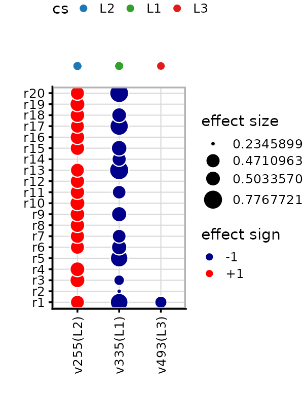

The first CS identifies a SNP affecting most traits, while the third CS identifies a SNP affecting only one trait.

Local false sign rate

The LFSR for a variable-trait pair gives the posterior probability that the estimated sign of the effect is wrong. Small LFSR values indicate confident effect identification. LFSR can be thought of as an alternative to a p-value, but is typically slightly more conservative.

cat("LFSR matrix dimensions:", dim(fit$lfsr), "\n")
cat("(rows = SNPs, columns = traits)\n\n")

# Show LFSR for SNPs in credible sets
for (cs_name in names(fit$sets$cs)) {
  sentinel <- fit$sets$cs[[cs_name]][which.max(
    fit$pip[fit$sets$cs[[cs_name]]])]
  n_sig <- sum(fit$lfsr[sentinel, ] < 0.01)
  cat(sprintf("%s sentinel (SNP %d): %d traits with LFSR < 0.01\n",
              cs_name, sentinel, n_sig))
}
# LFSR matrix dimensions: 1001 20 
# (rows = SNPs, columns = traits)
# 
# L1 sentinel (SNP 335): 14 traits with LFSR < 0.01
# L2 sentinel (SNP 255): 20 traits with LFSR < 0.01
# L3 sentinel (SNP 493): 0 traits with LFSR < 0.01

Single-effect LFSR gives the LFSR for each single effect (credible set) across traits:

cat("Single-effect LFSR dimensions:", dim(fit$single_effect_lfsr), "\n")
cat("(rows = effects, columns = traits)\n")
# Single-effect LFSR dimensions: 10 20 
# (rows = effects, columns = traits)

Outcome-specific PIPs

The overall PIP tells us whether a SNP affects any trait. The outcome-specific PIP tells us the probability that a SNP affects a specific trait. This is computed from the mixture weights and prior structure.

pip_po <- mvsusie_get_pip_per_outcome(fit)
cat("Per-outcome PIP matrix:", dim(pip_po), "\n")
# Per-outcome PIP matrix: 1001 20

# Compare overall PIP vs outcome-specific PIP for a few traits
traits_to_show <- c(1, 5, 10, 15)
pdat <- do.call(rbind, lapply(traits_to_show, function(t) {
  data.frame(overall_pip = fit$pip,
             outcome_pip = pip_po[, t],
             trait = paste0("Trait ", t))
}))
ggplot(pdat, aes(x = overall_pip, y = outcome_pip)) +
  geom_point(shape = 20, size = 1, color = "royalblue", alpha = 0.5) +
  geom_abline(intercept = 0, slope = 1, linetype = "dotted") +
  facet_wrap(~trait) +
  labs(x = "Overall PIP", y = "Outcome-specific PIP") +
  theme_cowplot(font_size = 10)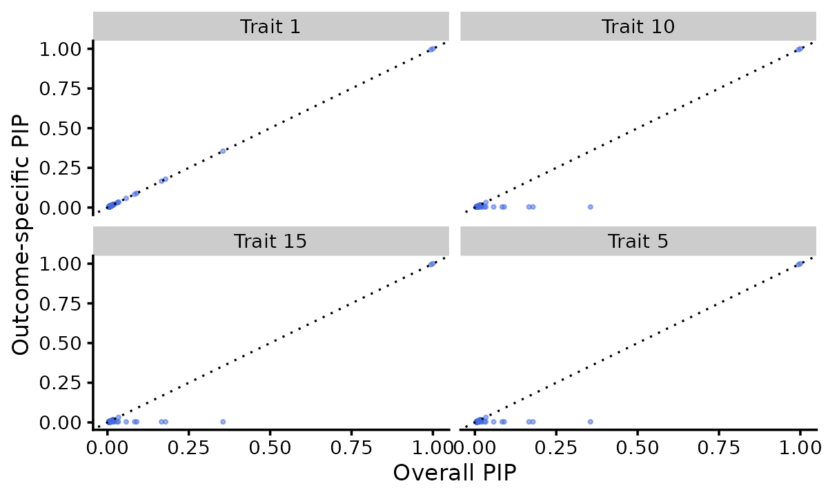

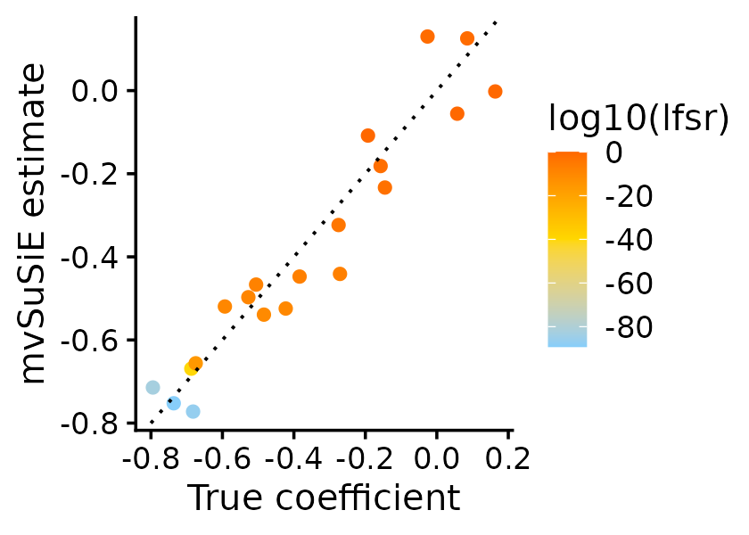
Per-effect coefficient estimates

Per-effect coefficient estimates on the original scale can be computed from alpha, mu, and X_column_scale_factors:

l <- 1
sentinel <- fit$sets$cs$L1[which.max(fit$pip[fit$sets$cs$L1])]
# Per-effect coefficient: alpha[l,j] * mu[l,j,r] / csd[j]
b_l <- fit$alpha[l, sentinel] * fit$mu[l, sentinel, ] /
       fit$X_column_scale_factors[sentinel]
pdat <- data.frame(
  true = simdata$Btrue[sentinel, ],
  estimated = b_l,
  lfsr = fit$single_effect_lfsr[l, ]
)
ggplot(pdat, aes(x = true, y = estimated,
                 color = log10(lfsr))) +
  geom_point(shape = 20, size = 2.5) +
  geom_abline(intercept = 0, slope = 1, linetype = "dotted") +
  scale_color_gradient2(low = "lightskyblue", mid = "gold",
                        high = "orangered", midpoint = -40) +
  labs(x = "True coefficient", y = "mvSuSiE estimate") +
  theme_cowplot(font_size = 12)