Introduction to mvSuSiE for multi-trait fine-mapping
Gao Wang
2026-05-17
Source:vignettes/mvsusie_intro.Rmd
mvsusie_intro.RmdThis vignette walks through the steps of a basic mvSuSiE multi-trait fine-mapping analysis using individual-level and summary data.
For detailed interpretation of the output including PIP, credible sets, LFSR, outcome-specific PIPs, and per-effect coefficient estimates, see the Interpreting and visualizing mvSuSiE results vignette.
First, load the necessary packages, and to ensure reproducibility set the seed.
Next, load the data set we will analyze.
data(simdata)The data consist of an N \times J
genotype matrix X and an N
\times R phenotype matrix Y where N=574 is the number of samples, J=1001 is the number of SNPs, and R=20 is the number of traits/phenotypes.
Specify the prior
Some care should be taken to choose the prior for your mvSuSiE analysis. To simplify the example we have defined the prior for you:
prior <- create_mixture_prior(list(matrices = simdata$par$U,
                                   weights = simdata$par$w),
                              null_weight = 0)
More generally, we recommend taking a “data-driven” approach to estimating the weights and the covariance matrices in the prior. For example, when there are many candidate fine-mapping regions in your study, you could fit the prior to all the top associations from each of the candidate fine-mapping regions. This data-driven approach is quite similar to the approach used in mashr, and we recommend looking through the vignettes in the mashr package for further guidance. See also the prior specification vignette.
Fit the mvSuSiE model
Now that we have set up the prior, we are ready to run mvsusie:
fit <- mvsusie(X,Y,standardize = TRUE,
               prior_variance = prior,
               residual_variance = simdata$par$V,
               estimate_prior_variance = TRUE)
# mvsusie: N=574, J=1001, R=20, L=10 [mem: 0.16 GB]
# Residual variance set, common_cov=TRUE [mem: 0.16 GB]
# Prior: K=19 mixture components [mem: 0.16 GB]
# Eigendecomposition cache: K=19, common_cov=TRUE [mem: 0.17 GB]
# Model initialized: J=1001, R=20, L=10, K=19 [mem: 0.17 GB]
# iter          ELBO       delta   sigma2      mem      V
#    1   -15961.8377           -   diag[0.845,1.08]   0.17 GB  [6.82e-02, 8.74e-03, 1.06e-01, 6.10e-04, 4.41e-04, 3.46e-04, 2.81e-04, 2.33e-04, 1.94e-04, 1.63e-04]
#    2   -15853.7500    1.08e+02   diag[0.833,0.996]   0.17 GB  [6.66e-02, 8.97e-03, 1.07e-01, 6.73e-05, 1.06e-04, 1.26e-04, 1.33e-04, 1.30e-04, 1.23e-04, 1.14e-04]
#    3   -15853.6586    9.14e-02   diag[0.833,0.997]   0.17 GB  [6.67e-02, 8.97e-03, 1.08e-01, 7.55e-05, 8.10e-05, 9.00e-05, 9.85e-05, 1.04e-04, 1.07e-04, 1.06e-04]
#    4   -15853.6578    8.31e-04   diag[0.834,0.997]   0.17 GB  [6.67e-02, 8.96e-03, 1.08e-01, 9.63e-05, 9.22e-05, 9.16e-05, 9.33e-05, 9.60e-05, 9.88e-05, 1.01e-04]
#    5   -15853.6577    6.51e-05   diag[0.834,0.997]   0.17 GB  [6.67e-02, 8.96e-03, 1.08e-01, 9.96e-05, 9.76e-05, 9.60e-05, 9.53e-05, 9.55e-05, 9.63e-05, 9.75e-05]  converged
In this call, we have provided mvSuSiE with the four key pieces of information needed to run the analysis: (1) the genotype matrix; (2) the phenotype matrix; (3) the prior on the effects; and (4) the residual variance-covariance matrix (an R \times R matrix).
The model identified the following credible sets:
mvSuSiE with summary data
mvsusieR also provides a “summary data” interface, building on the ideas developed in the susie-rss paper. Different combinations of summary statistics are accepted, but here we will focus on the most common case in which the z-scores from the association tests are used. These z-scores should be stored in a J \times R matrix:
Z <- simdata$sumstats$z
dim(Z)
# [1] 1001   20
In addition to the z-scores, the sample size and J \times J LD (correlation) matrix are needed. (Strictly speaking, the sample size is not required, but the estimates may be less accurate if the sample size is not provided.)
n <- simdata$sumstats$n
R <- simdata$sumstats$LD
Now we can fit an mvSuSiE model to these summary data via the
mvsusie_rss interface:
fit_rss <- mvsusie_rss(Z,R,n,
                       prior_variance = prior,
                       residual_variance = simdata$par$V,
                       estimate_prior_variance = TRUE)
# Eigendecomposition cache: K=19, common_cov=TRUE [mem: 0.20 GB]
# Model initialized: J=1001, R=20, L=10, K=19 [mem: 0.20 GB]
# iter          ELBO       delta   sigma2      mem      V
#    1   -15961.8377           -   diag[0.845,1.08]   0.20 GB  [6.82e-02, 8.74e-03, 1.06e-01, 6.10e-04, 4.41e-04, 3.46e-04, 2.81e-04, 2.33e-04, 1.94e-04, 1.63e-04]
#    2   -15958.2958    3.54e+00   diag[0.845,1.08]   0.20 GB  [6.67e-02, 9.24e-03, 1.06e-01, 2.09e-04, 2.18e-04, 2.05e-04, 1.86e-04, 1.66e-04, 1.48e-04, 1.31e-04]
#    3   -15958.2079    8.79e-02   diag[0.845,1.08]   0.20 GB  [6.68e-02, 9.22e-03, 1.07e-01, 1.34e-04, 1.57e-04, 1.68e-04, 1.68e-04, 1.62e-04, 1.52e-04, 1.41e-04]
#    4   -15958.2073    5.68e-04   diag[0.845,1.08]   0.20 GB  [6.68e-02, 9.22e-03, 1.07e-01, 1.39e-04, 1.45e-04, 1.52e-04, 1.58e-04, 1.59e-04, 1.56e-04, 1.51e-04]
#    5   -15958.2072    1.12e-04   diag[0.845,1.08]   0.20 GB  [6.68e-02, 9.22e-03, 1.07e-01, 1.47e-04, 1.46e-04, 1.48e-04, 1.51e-04, 1.54e-04, 1.55e-04, 1.53e-04]
#    6   -15958.2072    3.44e-05   diag[0.845,1.08]   0.20 GB  [6.68e-02, 9.22e-03, 1.07e-01, 1.51e-04, 1.49e-04, 1.49e-04, 1.50e-04, 1.51e-04, 1.53e-04, 1.53e-04]  converged
Comparing individual-level and summary data results
When the genotypes are standardized in mvsusie
(standardize = TRUE) and the LD estimates are obtained from
the same data that were used to compute the z-scores, both
mvsusie and mvsusie_rss give similar PIPs:
ggplot(data.frame(pip = fit$pip, pip_rss = fit_rss$pip),
       aes(x = pip, y = pip_rss)) +
  geom_point(shape = 20, size = 2, color = "royalblue") +
  geom_abline(intercept = 0, slope = 1, color = "black", linetype = "dotted") +
  labs(x = "mvsusie PIP", y = "mvsusie_rss PIP") +
  theme_cowplot(font_size = 12)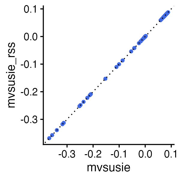
The PIPs are close but not identical because mvsusie()
defaults to estimate_residual_variance = TRUE
(re-estimating the residual variance from the data), whereas
mvsusie_rss() defaults to FALSE (since the
residual variance is difficult to estimate reliably from summary
statistics alone, as noted in Zou et
al.). For a detailed comparison of all input formats and the
effect of estimating the residual variance, see the input data formats vignette.
Of course, the results are also not always expected to be the same when the LD is estimated from an external reference panel.
Estimating the residual variance
In the above examples, we set the residual variance to the value that was used to simulate the data. In practice of course we will not have access to this so we will have to estimate the residual variance somehow.
When one has access to the summary data (specifically, the z-scores) for a large pool of independent SNPs that are expected to have little to no effect on the traits, one can use these z-scores to estimate the residual variance. Here, in this example data set, we do not have access to a large pool of independent “null SNPs”, but we can still use the data we have available to obtain a rough estimate of the residual variance. Specifically, we take as the “null SNPs” the SNPs in which the z-scores are all less than 2 in magnitude:
Z <- simdata$sumstats$z
null_markers <- which(apply(abs(Z),1,max) < 2)
length(null_markers)
Z <- Z[null_markers,]
Vest <- cov(Z)
# [1] 291
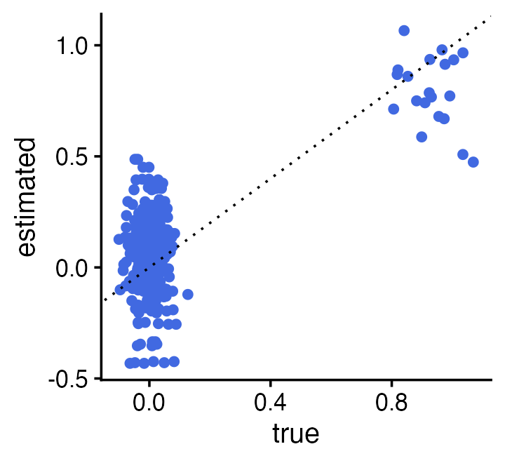
The estimate of the residual covariance matrix using these SNPs is reasonable, although presumably one could do better if we had the z-scores for more SNPs that were not in LD with the causal SNPs:
pdat <- data.frame(true = as.vector(simdata$par$V) + rnorm(400)/30,
                   estimated = as.vector(Vest))
ggplot(pdat,aes(x = true,y = estimated)) +
  geom_point(shape = 20,size = 2.5,color = "royalblue") +
  geom_abline(intercept = 0,slope = 1,color = "black",linetype = "dotted") +
  theme_cowplot(font_size = 12)