Engineering verification

Gao Wang

2026-05-17

This vignette verifies the internal consistency of the mvSuSiE implementation through two engineering checks: (1) the multivariate model reduces to univariate SuSiE when R = 1, and (2) the mixture prior code path agrees with the single-matrix code path when K = 1.

library(mvsusieR)
library(susieR)
library(ggplot2)
library(cowplot)
set.seed(1)

data(simdata)
X <- simdata$raw$X
n <- nrow(X); p <- ncol(X); r <- 10

B <- matrix(0, p, r)
causal <- sort(sample(p, 3))
for (j in causal) B[j, ] <- rnorm(r, 0, 0.5)
Y <- X %*% B + matrix(rnorm(n * r), n, r)

R = 1 reduces to univariate SuSiE

When there is only one outcome (R = 1), the multivariate model should give the same result as univariate SuSiE. This verifies that the multivariate code path correctly handles the scalar case.

Y1 <- Y[, 1]

# Univariate susie
fit_susie <- susie(X, Y1, L = 10,
                   scaled_prior_variance = 0.2,
                   tol = 1e-4)

# Multivariate mvsusie with R=1
fit_mv1 <- mvsusie(X, Y1, L = 10,
                   prior_variance = 0.2,
                   tol = 1e-4, verbose = FALSE)

cat("susie CS:", length(fit_susie$sets$cs), "\n")
cat("mvsusie (R=1) CS:", length(fit_mv1$sets$cs), "\n")
cat("max |PIP diff|:", max(abs(fit_susie$pip - fit_mv1$pip)), "\n")
# susie CS: 1 
# mvsusie (R=1) CS: 1 
# max |PIP diff|: 3.434324e-10

pdat <- data.frame(susie = fit_susie$pip, mvsusie = fit_mv1$pip)
ggplot(pdat, aes(x = susie, y = mvsusie)) +
  geom_point(shape = 20, size = 1.5, color = "royalblue", alpha = 0.5) +
  geom_abline(intercept = 0, slope = 1, linetype = "dotted") +
  labs(x = "PIP (susie)", y = "PIP (mvsusie, R=1)") +
  theme_cowplot(font_size = 12)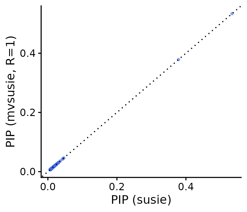

The PIPs agree at machine precision, confirming the R = 1 reduction.

Mixture prior (K > 1) vs single matrix prior (K = 1)

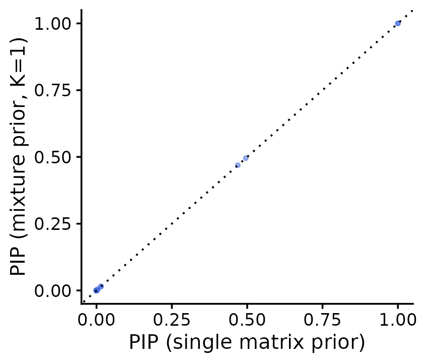
mvSuSiE supports two code paths for the prior: a single R \times R covariance matrix, and a mixture of K matrices (the “mash” prior). When K = 1, the mixture prior should give the same result as passing a single matrix directly. This verifies that the mixture machinery does not introduce any discrepancies.

U <- 0.2 * diag(r)

# Single matrix prior (K=1 code path)
fit_single <- mvsusie(X, Y, L = 10,
                      prior_variance = U,
                      residual_variance = diag(r),
                      max_iter = 100, tol = 1e-4, verbose = FALSE)

# Mixture prior with K=1 (mash code path)
prior_k1 <- create_mixture_prior(
  list(matrices = list(U), weights = 1)
)
fit_mixture <- mvsusie(X, Y, L = 10,
                       prior_variance = prior_k1,
                       residual_variance = diag(r),
                       max_iter = 100, tol = 1e-4, verbose = FALSE)

cat("Single matrix CS:", length(fit_single$sets$cs), "\n")
cat("Mixture (K=1) CS:", length(fit_mixture$sets$cs), "\n")
cat("max |PIP diff|:", max(abs(fit_single$pip - fit_mixture$pip)), "\n")
# Single matrix CS: 3 
# Mixture (K=1) CS: 3 
# max |PIP diff|: 0

pdat <- data.frame(single = fit_single$pip,
                   mixture = fit_mixture$pip)
ggplot(pdat, aes(x = single, y = mixture)) +
  geom_point(shape = 20, size = 1.5, color = "royalblue", alpha = 0.5) +
  geom_abline(intercept = 0, slope = 1, linetype = "dotted") +
  labs(x = "PIP (single matrix prior)",
       y = "PIP (mixture prior, K=1)") +
  theme_cowplot(font_size = 12)