Specifying and estimating priors in mvSuSiE

This vignette covers the choice of prior on effect sizes for mvSuSiE analysis from simplest naive approach (a fixed diagonal prior) to more flexible priors.

library(mvsusieR)
library(susieR)
library(ggplot2)
library(cowplot)
set.seed(1)

Simulate data

We use realistic genotypes and simulate 10 correlated traits with 4 causal SNPs.

data(simdata)
X <- simdata$raw$X
n <- nrow(X); p <- ncol(X); r <- 10

causal <- sort(sample(p, 4))
B <- matrix(0, p, r)
for (j in causal) B[j, ] <- rnorm(r, 0, 0.5)
Y <- X %*% B + matrix(rnorm(n * r), n, r)
cat(sprintf("Data: %d samples, %d SNPs, %d traits\n", n, p, r))
# Data: 574 samples, 1001 SNPs, 10 traits

Approach 1: Fixed diagonal prior

The simplest prior for getting started is a diagonal matrix scaled to represent the expected heritability per trait. Setting U = 0.2 \times \text{diag}(\text{var}(Y)) as initial value corresponds to approximately 20% heritability per trait under independent effects, assuming Y is standardized. This 20% will be updated by default with estimate_prior_variance = TRUE but the prior structure, the \text{diag}(\text{var}(Y)) part, will stay the same.

Y_var <- apply(Y, 2, var)
U_diag <- 0.2 * diag(Y_var)
prior_diag <- create_mixture_prior(
  list(matrices = list(U_diag), weights = 1)
)
cat("Prior type: single diagonal matrix\n")
cat("Number of components:", prior_diag$n_component, "\n")
# Prior type: single diagonal matrix
# Number of components:

fit_diag <- mvsusie(X, Y, L = 10,
                    prior_variance = prior_diag,
                    estimate_prior_variance = TRUE,
                    standardize = TRUE)
# mvsusie: N=574, J=1001, R=10, L=10 [mem: 0.16 GB]
# Residual variance set, common_cov=TRUE [mem: 0.17 GB]
# Prior: K=1 mixture components [mem: 0.17 GB]
# Eigendecomposition cache: K=1, common_cov=TRUE [mem: 0.17 GB]
# Model initialized: J=1001, R=10, L=10, K=1 [mem: 0.17 GB]
# iter          ELBO       delta   sigma2      mem      V
#    1    -8263.5332           -   diag[0.938,1.51]   0.17 GB  [4.88e-01, 1.49e-01, 8.89e-02, 0 x 7]
#    2    -8185.2200    7.83e+01   diag[0.862,1.09]   0.17 GB  [5.03e-01, 1.54e-01, 9.19e-02, 0 x 7]
#    3    -8185.2117    8.30e-03   diag[0.861,1.09]   0.17 GB  [5.03e-01, 1.54e-01, 9.20e-02, 0 x 7]
#    4    -8185.2117    4.20e-07   diag[0.861,1.09]   0.17 GB  [5.03e-01, 1.54e-01, 9.20e-02, 0 x 7]  converged
cat("Credible sets:", length(fit_diag$sets$cs), "\n")
# Credible sets: 3

Approach 2: Canonical mixture prior

A more flexible approach uses create_mixture_prior(R = r) which automatically generates a set of canonical covariance matrices. These include singleton matrices (effect in one trait only) and shared patterns with varying correlations.

prior_canon <- create_mixture_prior(R = r)
cat("Components:", prior_canon$n_component, "\n")
# Components:

fit_canon <- mvsusie(X, Y, L = 10,
                     prior_variance = prior_canon,
                     estimate_prior_variance = TRUE,
                     standardize = TRUE)
# mvsusie: N=574, J=1001, R=10, L=10 [mem: 0.17 GB]
# Residual variance set, common_cov=TRUE [mem: 0.17 GB]
# Prior: K=15 mixture components [mem: 0.17 GB]
# Eigendecomposition cache: K=15, common_cov=TRUE [mem: 0.17 GB]
# Model initialized: J=1001, R=10, L=10, K=15 [mem: 0.17 GB]
# iter          ELBO       delta   sigma2      mem      V
#    1    -8269.8068           -   diag[0.938,1.51]   0.18 GB  [1.48e-01, 3.88e-02, 2.44e-02, 0 x 7]
#    2    -8185.3120    8.45e+01   diag[0.862,1.09]   0.18 GB  [1.28e-01, 3.29e-02, 2.05e-02, 0 x 7]
#    3    -8185.3033    8.73e-03   diag[0.861,1.09]   0.18 GB  [1.28e-01, 3.29e-02, 2.05e-02, 0 x 7]
#    4    -8185.3033    4.16e-07   diag[0.861,1.09]   0.18 GB  [1.28e-01, 3.29e-02, 2.05e-02, 0 x 7]  converged
cat("Credible sets:", length(fit_canon$sets$cs), "\n")
# Credible sets: 3

Approach 3: Data-driven prior from mashr

For large-scale studies with many candidate regions, the recommended approach is to learn the prior from the data using mashr. The idea is to fit mashr to the top associations from each region, then use the fitted prior in mvSuSiE.

# Compute z-scores for mashr
Z <- calc_z(X, Y, center = TRUE, scale = TRUE)

# Set up mashr data
mash_data <- mashr::mash_set_data(Bhat = Z,
                                  Shat = matrix(1, p, r))

# Fit mashr (simplified for this example)
U_c <- mashr::cov_canonical(mash_data)
m_fit <- mashr::mash(mash_data, Ulist = U_c, outputlevel = 0)

# Create prior from mashr output
prior_mash <- create_mixture_prior(fitted_g = m_fit$fitted_g)
cat("Components from mashr:", prior_mash$n_component, "\n")
#  - Computing 1001 x 271 likelihood matrix.
#  - Likelihood calculations took 0.04 seconds.
#  - Fitting model with 271 mixture components.
#  - Model fitting took 0.44 seconds.
# Components from mashr:

fit_mash <- mvsusie(X, Y, L = 10,
                    prior_variance = prior_mash,
                    estimate_prior_variance = TRUE,
                    standardize = TRUE)
# mvsusie: N=574, J=1001, R=10, L=10 [mem: 0.17 GB]
# Residual variance set, common_cov=TRUE [mem: 0.18 GB]
# Prior: K=8 mixture components [mem: 0.18 GB]
# Eigendecomposition cache: K=8, common_cov=TRUE [mem: 0.18 GB]
# Model initialized: J=1001, R=10, L=10, K=8 [mem: 0.18 GB]
# iter          ELBO       delta   sigma2      mem      V
#    1    -8268.5177           -   diag[0.938,1.51]   0.18 GB  [1.09e-01, 2.76e-02, 1.70e-02, 0 x 7]
#    2    -8185.3118    8.32e+01   diag[0.862,1.09]   0.18 GB  [1.21e-01, 3.11e-02, 1.94e-02, 0 x 7]
#    3    -8185.3033    8.51e-03   diag[0.861,1.09]   0.18 GB  [1.21e-01, 3.12e-02, 1.94e-02, 0 x 7]
#    4    -8185.3033    4.02e-07   diag[0.861,1.09]   0.18 GB  [1.21e-01, 3.12e-02, 1.94e-02, 0 x 7]  converged
cat("Credible sets:", length(fit_mash$sets$cs), "\n")
# Credible sets: 3

Comparing priors

pdat <- data.frame(
  pip = c(fit_diag$pip, fit_canon$pip, fit_mash$pip),
  prior = rep(c("Diagonal", "Canonical", "mashr"),
              each = p),
  pos = rep(seq_len(p), 3)
)
ggplot(pdat, aes(x = pos, y = pip)) +
  geom_point(shape = 20, size = 1, color = "royalblue", alpha = 0.5) +
  facet_wrap(~prior) +
  geom_vline(xintercept = causal, linetype = "dashed",
             color = "red", alpha = 0.5) +
  labs(x = "SNP position", y = "PIP") +
  theme_cowplot(font_size = 10)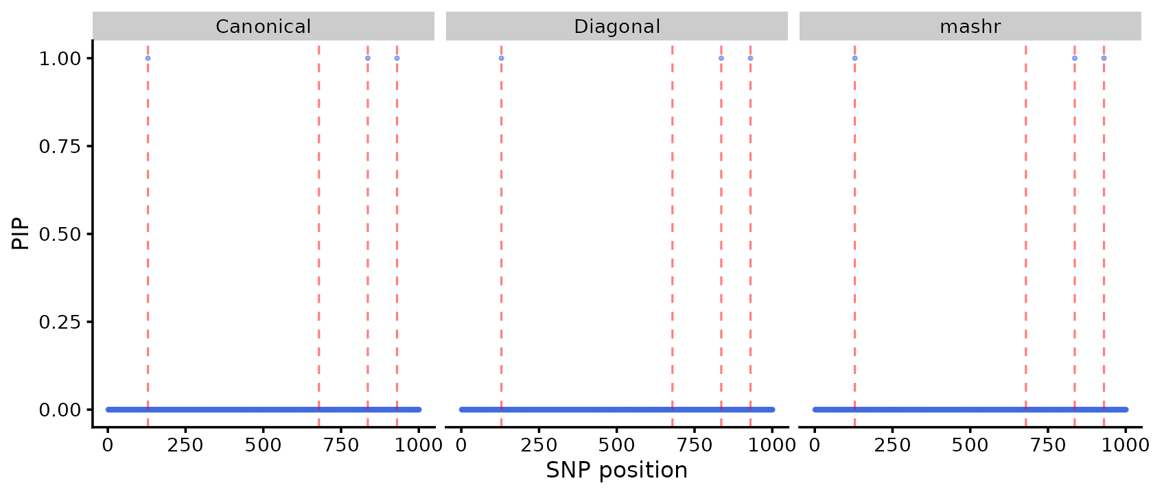

All three priors identify the causal variants (red dashed lines) for this trivial example, but in practice the mixture priors can provide better trait-specific resolution, as shown in Zou et al (2026).

Mixture weight estimation

When using a mixture prior, the estimate_prior_mixture_weights option (default TRUE) allows the relative weights of the mixture components to be estimated from the data. This is useful for pruning irrelevant components and adapting to the data.

fit_fixed_w <- mvsusie(X, Y, L = 10,
                       prior_variance = prior_canon,
                       estimate_prior_variance = TRUE,
                       estimate_prior_mixture_weights = FALSE,
                       standardize = TRUE, verbose = FALSE)
fit_est_w <- mvsusie(X, Y, L = 10,
                     prior_variance = prior_canon,
                     estimate_prior_variance = TRUE,
                     estimate_prior_mixture_weights = TRUE,
                     standardize = TRUE, verbose = FALSE)
cat("Fixed weights ELBO:", tail(fit_fixed_w$elbo, 1), "\n")
cat("Estimated weights ELBO:", tail(fit_est_w$elbo, 1), "\n")
cat("(Higher ELBO is better)\n")
# Fixed weights ELBO: -8191.489 
# Estimated weights ELBO: -8185.303 
# (Higher ELBO is better)

The weight estimation method can be set via mixture_weight_method: "mixsqp" (default, uses the mixsqp package for fast optimization) or "EM". The former might be slower per iteration but the latter might take longer to converge.