Per-trait sample sizes in mvSuSiE RSS

When combining summary statistics from different studies — for example, a GWAS trait (N = 300\text{K}) and an eQTL trait (N = 700) — each trait has its own sample size. The z-score-only interface to mvsusie_rss() takes a single scalar N and constructs sufficient statistics as X^TX = (N-1)\,R and X^TY = \sqrt{N-1}\,Z. It cannot represent this difference directly.
Because mvSuSiE RSS assumes a shared LD structure across all traits, which is reasonable when all studies are from the same ancestry, even if their sample sizes differ.

This vignette shows a workaround converting z-scores with per-trait sample sizes into Bhat/Shat inputs that at least will encode the per-trait uncertainty into standard error, such that traits with smaller N get larger standard errors, which correctly reduces their influence on the posterior.

library(mvsusieR)
library(susieR)
library(ggplot2)
library(cowplot)
set.seed(1)

We simulate 5 traits on the same genotypes, then assign different “effective” sample sizes to each trait to mimic the scenario where z-scores come from studies of different sizes.

data(simdata)
X <- simdata$raw$X
n <- nrow(X)
p <- ncol(X)
r <- 5
cat(sprintf("Genotype matrix: %d samples x %d SNPs\n", n, p))

causal <- sort(sample(p, 3))
B <- matrix(0, p, r)
for (j in causal) B[j, ] <- rnorm(r, 0, 0.5)
Y <- X %*% B + matrix(rnorm(n * r), n, r)
cat("Causal SNPs:", causal, "\n")

# Per-trait sample sizes: traits 1-2 use full data,
# traits 3-4 are moderate, trait 5 is small (eQTL-like).
N_vec <- c(n, n, round(n / 5), round(n / 5), round(n / 20))
cat("Per-trait N:", N_vec, "\n")
# Genotype matrix: 574 samples x 1001 SNPs
# Causal SNPs: 129 679 836 
# Per-trait N: 574 574 115 115 29

prior <- create_mixture_prior(R = r)
resid_var <- diag(r)
Z <- calc_z(X, Y, center = TRUE, scale = TRUE)
LD <- cor(X)

Convert z-scores to Bhat / Shat

On the standardized scale (\mathrm{var}(X_j) = 1, \mathrm{var}(Y_r) = 1), the marginal z-score follows a t-distribution with N_r - 2 degrees of freedom. The exact conversion is:

\mathrm{Shat}_{jr} = \frac{1}{\sqrt{N_r - 2 + Z_{jr}^2}}, \qquad \mathrm{Bhat}_{jr} = Z_{jr}\;\mathrm{Shat}_{jr}.

For large N_r and moderate Z this simplifies to \mathrm{Shat} \approx 1/\sqrt{N_r} and \mathrm{Bhat} \approx Z/\sqrt{N_r}. The exact form is preferred when N_r is small or |Z| is large, because it properly accounts for the finite-sample PVE adjustment.

Bhat <- matrix(0, p, r)
Shat <- matrix(0, p, r)
for (rr in seq_len(r)) {
  denom <- sqrt(N_vec[rr] - 2 + Z[, rr]^2)
  Bhat[, rr] <- Z[, rr] / denom
  Shat[, rr] <- 1 / denom
}

cat("Shat magnitude at a null SNP (SNP 1):\n")
cat("  per trait:", round(Shat[1, ], 4), "\n")
cat("  ratio to max-N trait:", round(Shat[1, ] / Shat[1, 1], 2), "\n")
# Shat magnitude at a null SNP (SNP 1):
#   per trait: 0.0417 0.0417 0.094 0.0938 0.1895 
#   ratio to max-N trait: 1 1 2.25 2.25 4.54

Traits with smaller N get larger standard errors (roughly \sqrt{N_{\max}/N_r} times larger).

Fit with per-trait sample sizes

Pass Bhat, Shat, and a varY to mvsusie_rss(). In our simulation on the standardized scale, varY is an identity matrix, but in practice this can be left unspecified so that the residual correlation is estimated internally from null z-scores. We use estimate_residual_variance = FALSE (the default for summary statistics).

Notice that mvsusie_rss() still requires a scalar N. Inside the function, N is used for the PVE adjustment (cf Zou 2022). We pass N = max(N_vec) so that the large-N traits (which dominate discovery) get the correct adjustment. For the small-N traits the PVE correction is slightly too weak but the primary sample-size information is already encoded in Shat, which correctly inflates the standard errors:

varY_id <- diag(r)

# Per-trait N via Bhat/Shat conversion
fit_diff <- mvsusie_rss(Bhat = Bhat, Shat = Shat, R = LD,
                         N = max(N_vec), varY = varY_id, L = 10,
                         prior_variance = prior,
                         residual_variance = resid_var,
                         estimate_residual_variance = FALSE,
                         estimate_prior_variance = TRUE)
# Eigendecomposition cache: K=10, common_cov=TRUE [mem: 0.19 GB]
# Model initialized: J=1001, R=5, L=10, K=10 [mem: 0.19 GB]
# iter          ELBO       delta   sigma2      mem      V
#    1    -3875.7987           -   diag[1,1]   0.20 GB  [1.15e-01, 9.65e-02, 0 x 8]
#    2    -3872.5371    3.26e+00   diag[1,1]   0.20 GB  [9.18e-02, 7.39e-02, 0 x 8]
#    3    -3872.5371    1.07e-05   diag[1,1]   0.20 GB  [9.19e-02, 7.39e-02, 0 x 8]  converged
# WARNING: Xcorr is not symmetric; using (Xcorr + t(Xcorr))/2.

# Baseline: same N for all traits (ignoring the difference)
Bhat0 <- Shat0 <- matrix(0, p, r)
for (rr in seq_len(r)) {
  denom <- sqrt(n - 2 + Z[, rr]^2)
  Bhat0[, rr] <- Z[, rr] / denom
  Shat0[, rr] <- 1 / denom
}
fit_same <- mvsusie_rss(Bhat = Bhat0, Shat = Shat0, R = LD,
                         N = n, varY = varY_id, L = 10,
                         prior_variance = prior,
                         residual_variance = resid_var,
                         estimate_residual_variance = FALSE,
                         estimate_prior_variance = TRUE)
# Eigendecomposition cache: K=10, common_cov=TRUE [mem: 0.20 GB]
# Model initialized: J=1001, R=5, L=10, K=10 [mem: 0.20 GB]
# iter          ELBO       delta   sigma2      mem      V
#    1    -3957.2010           -   diag[1,1]   0.20 GB  [7.54e-02, 5.98e-02, 0 x 8]
#    2    -3953.9390    3.26e+00   diag[1,1]   0.20 GB  [5.94e-02, 4.55e-02, 0 x 8]
#    3    -3953.9390    8.43e-06   diag[1,1]   0.20 GB  [5.94e-02, 4.55e-02, 0 x 8]  converged
# WARNING: Xcorr is not symmetric; using (Xcorr + t(Xcorr))/2.

Compare results

The PIPs and credible sets are similar because variable selection is driven primarily by the large-N traits.

cat("Credible sets (same N):", length(fit_same$sets$cs), "\n")
cat("Credible sets (diff N):", length(fit_diff$sets$cs), "\n")
cat("PIP correlation:", round(cor(fit_same$pip, fit_diff$pip), 4), "\n")
# Credible sets (same N): 2 
# Credible sets (diff N): 2 
# PIP correlation: 1

However, traits with smaller N produce larger (less confident) LFSR values:

trait_labels <- paste0("Trait ", 1:r, " (N=", N_vec, ")")
cat("Single-effect LFSR per credible set:\n\n")
for (i in seq_along(fit_same$sets$cs)) {
  cs_name <- names(fit_same$sets$cs)[i]
  cat(cs_name, ":\n")
  lfsr_s <- fit_same$single_effect_lfsr[i, ]
  lfsr_d <- fit_diff$single_effect_lfsr[i, ]
  for (rr in 1:r) {
    flag <- if (lfsr_d[rr] > lfsr_s[rr] + 0.01) " *" else ""
    cat(sprintf("  %-20s  same=%.4f  diff=%.4f%s\n",
                trait_labels[rr], lfsr_s[rr], lfsr_d[rr], flag))
  }
  cat("\n")
}
# Single-effect LFSR per credible set:
# 
# L1 :
#   Trait 1 (N=574)       same=0.0000  diff=0.0000
#   Trait 2 (N=574)       same=0.0000  diff=0.0000
#   Trait 3 (N=115)       same=1.0000  diff=1.0000
#   Trait 4 (N=115)       same=0.0000  diff=0.0005
#   Trait 5 (N=29)        same=0.0000  diff=1.0000 *
# 
# L2 :
#   Trait 1 (N=574)       same=0.0008  diff=0.0000
#   Trait 2 (N=574)       same=0.0000  diff=0.0000
#   Trait 3 (N=115)       same=0.0000  diff=0.0000
#   Trait 4 (N=115)       same=1.0000  diff=1.0000
#   Trait 5 (N=29)        same=1.0000  diff=1.0000

Entries marked with * show traits where the per-trait N correctly increases the LFSR.

# Gather LFSR for all effects into a data frame
lfsr_list <- list()
for (i in seq_along(fit_same$sets$cs)) {
  cs_name <- names(fit_same$sets$cs)[i]
  lfsr_list[[length(lfsr_list) + 1]] <- data.frame(
    lfsr_same = fit_same$single_effect_lfsr[i, ],
    lfsr_diff = fit_diff$single_effect_lfsr[i, ],
    trait = trait_labels,
    cs = cs_name, stringsAsFactors = FALSE)
}
lfsr_dat <- do.call(rbind, lfsr_list)
lfsr_dat$trait <- factor(lfsr_dat$trait, levels = trait_labels)

ggplot(lfsr_dat, aes(x = lfsr_same, y = lfsr_diff, color = trait)) +
  geom_point(size = 3) +
  geom_abline(intercept = 0, slope = 1, linetype = "dotted") +
  scale_color_brewer(palette = "Set1") +
  labs(x = "LFSR (same N for all traits)",
       y = "LFSR (per-trait N)",
       color = "") +
  theme_cowplot(font_size = 11) +
  theme(legend.position = "right")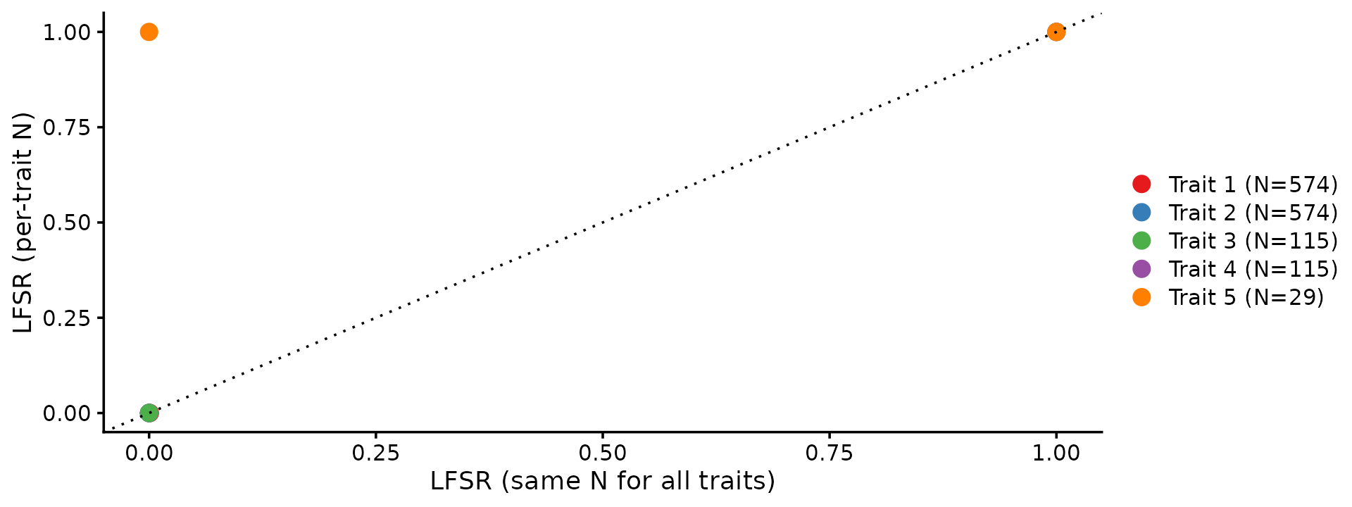

Points above the diagonal are traits where using per-trait N makes the model less confident, which is the correct behavior for traits with smaller sample sizes.

Gao Wang

2026-05-17

Convert z-scores to Bhat / Shat

Fit with per-trait sample sizes

Compare results