Handling missing data in mvSuSiE
Gao Wang
2026-05-17
Source:vignettes/missing_data.Rmd
missing_data.RmdmvSuSiE can handle missing values in the phenotype matrix Y. This is useful in two common scenarios:
Random missing data (MCAR): individual measurements are randomly missing across samples and traits.
Block missing data: entire traits are unobserved for subsets of samples. This arises naturally in cross-population or cross-ancestry analyses where different cohorts measure different traits.
The default method missing_y_method = "approximate" as
described in Zou’s
thesis (2021) handles both scenarios. An alternative
"impute" method, as discussed in Zou et al
(2026) is available and may perform well for MCAR with lower missing
values, but loses power for block-structured missingness (see
below).
Simulate complete data
data(simdata)
X <- simdata$raw$X
n <- nrow(X); p <- ncol(X); r <- 10

causal <- sort(sample(p, 4))
B <- matrix(0, p, r)
for (j in causal) B[j, ] <- rnorm(r, 0, 0.5)
Y_complete <- X %*% B + matrix(rnorm(n * r), n, r)
cat(sprintf("Complete data: %d x %d x %d (N x J x R)\n", n, p, r))
cat("True causal SNPs:", causal, "\n")
# Complete data: 574 x 1001 x 10 (N x J x R)
# True causal SNPs: 129 679 836 930
Fit the model on complete data for reference.
prior <- create_mixture_prior(R = r)
fit_complete <- mvsusie(X, Y_complete, L = 10,
                        prior_variance = prior)
# mvsusie: N=574, J=1001, R=10, L=10 [mem: 0.16 GB]
# Residual variance set, common_cov=TRUE [mem: 0.17 GB]
# Prior: K=15 mixture components [mem: 0.17 GB]
# Eigendecomposition cache: K=15, common_cov=TRUE [mem: 0.17 GB]
# Model initialized: J=1001, R=10, L=10, K=15 [mem: 0.17 GB]
# iter          ELBO       delta   sigma2      mem      V
#    1    -8269.8068           -   diag[0.938,1.51]   0.17 GB  [1.48e-01, 3.88e-02, 2.44e-02, 0 x 7]
#    2    -8185.3120    8.45e+01   diag[0.862,1.09]   0.17 GB  [1.28e-01, 3.29e-02, 2.05e-02, 0 x 7]
#    3    -8185.3033    8.73e-03   diag[0.861,1.09]   0.17 GB  [1.28e-01, 3.29e-02, 2.05e-02, 0 x 7]
#    4    -8185.3033    4.16e-07   diag[0.861,1.09]   0.17 GB  [1.28e-01, 3.29e-02, 2.05e-02, 0 x 7]  converged
cat("Complete data: CS =", length(fit_complete$sets$cs), "\n")
# Complete data: CS = 3
We evaluate performance at the credible set (CS) level: a true positive is a CS that contains at least one causal SNP; a false positive is a CS containing no causal SNP.
check_cs <- function(fit, causal, label) {
  cs_list <- fit$sets$cs
  n_cs <- if (is.null(cs_list)) 0 else length(cs_list)
  tp <- 0; fp <- 0
  if (n_cs > 0) {
    for (i in seq_along(cs_list)) {
      if (any(cs_list[[i]] %in% causal)) tp <- tp + 1
      else fp <- fp + 1
    }
  }
  captured <- sapply(causal, function(c) {
    any(sapply(cs_list, function(cs) c %in% cs))
  })
  cat(sprintf("%s: %d CS (%d true, %d false), %d/%d causal captured\n",
              label, n_cs, tp, fp, sum(captured), length(causal)))
}
check_cs(fit_complete, causal, "Complete")
# Complete: 3 CS (3 true, 0 false), 3/4 causal captured
Random missing data (MCAR)
We introduce missing values completely at random at three rates: 5%, 20%, and 50%.
insert_random_na <- function(Y, frac) {
  Y_miss <- Y
  n_miss <- round(frac * length(Y))
  idx <- sample(length(Y), n_miss)
  Y_miss[idx] <- NA
  Y_miss
}

Y_miss_05 <- insert_random_na(Y_complete, 0.05)
Y_miss_20 <- insert_random_na(Y_complete, 0.20)
Y_miss_50 <- insert_random_na(Y_complete, 0.50)
cat("Missing values: 5% =", sum(is.na(Y_miss_05)),
    ", 20% =", sum(is.na(Y_miss_20)),
    ", 50% =", sum(is.na(Y_miss_50)), "\n")
# Missing values: 5% = 287 , 20% = 1148 , 50% = 2870
Default method (approximate)
fit_05 <- mvsusie(X, Y_miss_05, L = 10, prior_variance = prior)
# mvsusie: N=574, J=1001, R=10, L=10 [mem: 0.17 GB]
# Residual variance set, common_cov=FALSE [mem: 0.22 GB]
# Prior: K=15 mixture components [mem: 0.22 GB]
# Eigendecomposition cache: K=15, common_cov=FALSE [mem: 0.25 GB]
# Model initialized: J=1001, R=10, L=10, K=15 [mem: 0.25 GB]
# iter          ELBO       delta   sigma2      mem      V
#    1    -7863.5517           -   diag[0.959,1.52]   0.25 GB  [1.52e-01, 3.96e-02, 2.74e-02, 0 x 7]
#    2    -7857.2236    6.33e+00   diag[0.959,1.52]   0.25 GB  [1.27e-01, 3.29e-02, 2.23e-02, 0 x 7]
#    3    -7857.2234    1.59e-04   diag[0.959,1.52]   0.25 GB  [1.27e-01, 3.29e-02, 2.23e-02, 0 x 7]
#    4    -7857.2234    1.01e-08   diag[0.959,1.52]   0.25 GB  [1.27e-01, 3.29e-02, 2.23e-02, 0 x 7]  converged
# Eigendecomposition cache: K=15, common_cov=FALSE [mem: 0.25 GB]
# Model initialized: J=1001, R=10, L=10, K=15 [mem: 0.25 GB]
# iter          ELBO       delta   sigma2      mem      V
#    1    -7786.5887           -   diag[0.85,1.1]   0.25 GB  [1.56e-01, 4.11e-02, 2.77e-02, 0 x 7]
#    2    -7780.4774    6.11e+00   diag[0.85,1.1]   0.25 GB  [1.31e-01, 3.38e-02, 2.26e-02, 0 x 7]
#    3    -7780.4772    1.76e-04   diag[0.85,1.1]   0.25 GB  [1.31e-01, 3.38e-02, 2.26e-02, 0 x 7]
#    4    -7780.4772    8.39e-09   diag[0.85,1.1]   0.25 GB  [1.31e-01, 3.38e-02, 2.26e-02, 0 x 7]  converged
# Block ascent iter 1: ELBO=-7780.4772, change=76.75, sigma2=[1, 1.032, 1.028, 1.038, 0.911, 0.85, 1.028, 1.004, 1.103, 1.014]
# Eigendecomposition cache: K=15, common_cov=FALSE [mem: 0.26 GB]
# Model initialized: J=1001, R=10, L=10, K=15 [mem: 0.26 GB]
# iter          ELBO       delta   sigma2      mem      V
#    1    -7786.5800           -   diag[0.849,1.1]   0.26 GB  [1.56e-01, 4.12e-02, 2.77e-02, 0 x 7]
#    2    -7780.4694    6.11e+00   diag[0.849,1.1]   0.26 GB  [1.31e-01, 3.38e-02, 2.26e-02, 0 x 7]
#    3    -7780.4692    1.77e-04   diag[0.849,1.1]   0.26 GB  [1.31e-01, 3.38e-02, 2.26e-02, 0 x 7]
#    4    -7780.4692    8.43e-09   diag[0.849,1.1]   0.26 GB  [1.31e-01, 3.38e-02, 2.26e-02, 0 x 7]  converged
# Block ascent iter 2: ELBO=-7780.4692, change=0.007997, sigma2=[0.999, 1.032, 1.027, 1.037, 0.911, 0.849, 1.025, 1.003, 1.102, 1.013]
fit_20 <- mvsusie(X, Y_miss_20, L = 10, prior_variance = prior)
# mvsusie: N=574, J=1001, R=10, L=10 [mem: 0.17 GB]
# Residual variance set, common_cov=FALSE [mem: 0.23 GB]
# Prior: K=15 mixture components [mem: 0.23 GB]
# Eigendecomposition cache: K=15, common_cov=FALSE [mem: 0.25 GB]
# Model initialized: J=1001, R=10, L=10, K=15 [mem: 0.25 GB]
# iter          ELBO       delta   sigma2      mem      V
#    1    -6622.3736           -   diag[0.933,1.53]   0.25 GB  [1.50e-01, 4.22e-02, 2.16e-02, 7.60e-03, 0 x 6]
#    2    -6615.6217    6.75e+00   diag[0.933,1.53]   0.25 GB  [1.33e-01, 3.63e-02, 1.83e-02, 7.60e-03, 0 x 6]
#    3    -6615.5952    2.65e-02   diag[0.933,1.53]   0.25 GB  [1.29e-01, 3.53e-02, 1.81e-02, 7.60e-03, 0 x 6]
#    4    -6615.5942    9.44e-04   diag[0.933,1.53]   0.25 GB  [1.29e-01, 3.52e-02, 1.81e-02, 7.60e-03, 0 x 6]
#    5    -6615.5942    2.68e-05   diag[0.933,1.53]   0.25 GB  [1.29e-01, 3.51e-02, 1.80e-02, 7.60e-03, 0 x 6]  converged
# Eigendecomposition cache: K=15, common_cov=FALSE [mem: 0.26 GB]
# Model initialized: J=1001, R=10, L=10, K=15 [mem: 0.26 GB]
# iter          ELBO       delta   sigma2      mem      V
#    1    -6562.8330           -   diag[0.828,1.08]   0.26 GB  [1.56e-01, 4.32e-02, 2.29e-02, 8.56e-03, 0 x 6]
#    2    -6556.1480    6.69e+00   diag[0.828,1.08]   0.26 GB  [1.41e-01, 3.81e-02, 1.95e-02, 7.47e-03, 0 x 6]
#    3    -6556.1241    2.39e-02   diag[0.828,1.08]   0.26 GB  [1.37e-01, 3.70e-02, 1.92e-02, 7.63e-03, 0 x 6]
#    4    -6556.1223    1.78e-03   diag[0.828,1.08]   0.26 GB  [1.36e-01, 3.68e-02, 1.91e-02, 7.68e-03, 0 x 6]
#    5    -6556.1222    1.05e-04   diag[0.828,1.08]   0.26 GB  [1.35e-01, 3.67e-02, 1.91e-02, 7.70e-03, 0 x 6]
#    6    -6556.1222    5.75e-06   diag[0.828,1.08]   0.26 GB  [1.35e-01, 3.67e-02, 1.91e-02, 7.70e-03, 0 x 6]  converged
# Block ascent iter 1: ELBO=-6556.1222, change=59.47, sigma2=[0.973, 1.027, 1.047, 1.075, 0.886, 0.828, 1.008, 1.029, 1.054, 1.05]
# Eigendecomposition cache: K=15, common_cov=FALSE [mem: 0.26 GB]
# Model initialized: J=1001, R=10, L=10, K=15 [mem: 0.26 GB]
# iter          ELBO       delta   sigma2      mem      V
#    1    -6562.8301           -   diag[0.827,1.07]   0.26 GB  [1.56e-01, 4.32e-02, 2.29e-02, 8.59e-03, 0 x 6]
#    2    -6556.1443    6.69e+00   diag[0.827,1.07]   0.26 GB  [1.41e-01, 3.82e-02, 1.96e-02, 7.49e-03, 0 x 6]
#    3    -6556.1208    2.34e-02   diag[0.827,1.07]   0.26 GB  [1.37e-01, 3.71e-02, 1.93e-02, 7.65e-03, 0 x 6]
#    4    -6556.1191    1.76e-03   diag[0.827,1.07]   0.26 GB  [1.36e-01, 3.68e-02, 1.92e-02, 7.70e-03, 0 x 6]
#    5    -6556.1190    1.04e-04   diag[0.827,1.07]   0.26 GB  [1.35e-01, 3.68e-02, 1.91e-02, 7.71e-03, 0 x 6]
#    6    -6556.1190    5.74e-06   diag[0.827,1.07]   0.26 GB  [1.35e-01, 3.67e-02, 1.91e-02, 7.71e-03, 0 x 6]  converged
# Block ascent iter 2: ELBO=-6556.1190, change=0.00323, sigma2=[0.972, 1.027, 1.045, 1.074, 0.884, 0.827, 1.004, 1.028, 1.054, 1.049]
fit_50 <- mvsusie(X, Y_miss_50, L = 10, prior_variance = prior)
# mvsusie: N=574, J=1001, R=10, L=10 [mem: 0.18 GB]
# Warning: Cholesky failed for 10x10 matrix; falling back to SVD pseudo-inverse
# Residual variance set, common_cov=FALSE [mem: 0.23 GB]
# Prior: K=15 mixture components [mem: 0.23 GB]
# Eigendecomposition cache: K=15, common_cov=FALSE [mem: 0.26 GB]
# Model initialized: J=1001, R=10, L=10, K=15 [mem: 0.26 GB]
# iter          ELBO       delta   sigma2      mem      V
#    1    -4113.8308           -   diag[0.926,1.54]   0.26 GB  [1.44e-01, 3.65e-02, 2.29e-02, 0 x 7]
#    2    -4107.1905    6.64e+00   diag[0.926,1.54]   0.26 GB  [1.22e-01, 2.85e-02, 1.93e-02, 0 x 7]
#    3    -4107.1896    8.89e-04   diag[0.926,1.54]   0.26 GB  [1.21e-01, 2.85e-02, 1.93e-02, 0 x 7]
#    4    -4107.1896    7.28e-07   diag[0.926,1.54]   0.26 GB  [1.21e-01, 2.85e-02, 1.93e-02, 0 x 7]  converged
# Eigendecomposition cache: K=15, common_cov=FALSE [mem: 0.27 GB]
# Model initialized: J=1001, R=10, L=10, K=15 [mem: 0.27 GB]
# iter          ELBO       delta   sigma2      mem      V
#    1    -4076.6402           -   diag[0.816,1.11]   0.27 GB  [1.56e-01, 3.58e-02, 2.64e-02, 0 x 7]
#    2    -4070.3633    6.28e+00   diag[0.816,1.11]   0.27 GB  [1.31e-01, 2.93e-02, 2.16e-02, 0 x 7]
#    3    -4070.3630    3.65e-04   diag[0.816,1.11]   0.27 GB  [1.31e-01, 2.93e-02, 2.16e-02, 0 x 7]
#    4    -4070.3630    3.12e-07   diag[0.816,1.11]   0.27 GB  [1.31e-01, 2.93e-02, 2.16e-02, 0 x 7]  converged
# Block ascent iter 1: ELBO=-4070.3630, change=36.83, sigma2=[0.897, 1.091, 0.883, 1.083, 0.909, 0.816, 1.031, 1.007, 1.107, 0.972]
# Eigendecomposition cache: K=15, common_cov=FALSE [mem: 0.27 GB]
# Model initialized: J=1001, R=10, L=10, K=15 [mem: 0.27 GB]
# iter          ELBO       delta   sigma2      mem      V
#    1    -4076.5856           -   diag[0.814,1.11]   0.27 GB  [1.57e-01, 3.57e-02, 2.66e-02, 0 x 7]
#    2    -4070.3100    6.28e+00   diag[0.814,1.11]   0.27 GB  [1.32e-01, 2.93e-02, 2.17e-02, 0 x 7]
#    3    -4070.3096    3.95e-04   diag[0.814,1.11]   0.27 GB  [1.32e-01, 2.93e-02, 2.17e-02, 0 x 7]
#    4    -4070.3096    3.65e-07   diag[0.814,1.11]   0.27 GB  [1.32e-01, 2.93e-02, 2.17e-02, 0 x 7]  converged
# Block ascent iter 2: ELBO=-4070.3096, change=0.05333, sigma2=[0.895, 1.09, 0.878, 1.081, 0.909, 0.814, 1.025, 1.005, 1.106, 0.971]
# WARNING: "Cholesky failed for 10x10 matrix; falling back to SVD pseudo-inverse" occurred 3 times total (2 suppressed)
check_cs(fit_05, causal, "5% missing (approx)")
check_cs(fit_20, causal, "20% missing (approx)")
check_cs(fit_50, causal, "50% missing (approx)")
# 5% missing (approx): 3 CS (3 true, 0 false), 3/4 causal captured
# 20% missing (approx): 4 CS (4 true, 0 false), 4/4 causal captured
# 50% missing (approx): 3 CS (3 true, 0 false), 3/4 causal captured
pdat <- data.frame(
  complete = rep(fit_complete$pip, 3),
  missing = c(fit_05$pip, fit_20$pip, fit_50$pip),
  frac = rep(c("5% missing", "20% missing", "50% missing"), each = p)
)
ggplot(pdat, aes(x = complete, y = missing)) +
  geom_point(shape = 20, size = 1.5, color = "royalblue", alpha = 0.5) +
  geom_abline(intercept = 0, slope = 1, linetype = "dotted") +
  facet_wrap(~frac) +
  labs(x = "PIP (complete data)", y = "PIP (approximate)") +
  theme_cowplot(font_size = 10)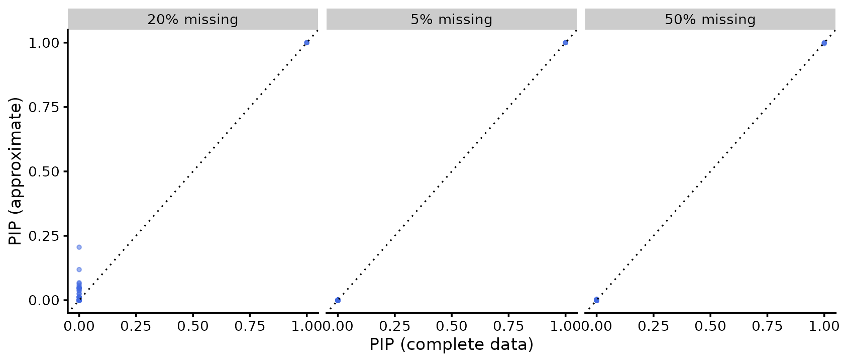
With moderate amounts of missing data, the default
"approximate" method gives results largely similar to the
complete data analysis, although some signs of inflation in PIP can be
observed in this experiments.
Impute method
The "impute" method also handles MCAR data well:
fit_imp_05 <- mvsusie(X, Y_miss_05, L = 10, prior_variance = prior,
                      missing_y_method = "impute")
# mvsusie: N=574, J=1001, R=10, L=10 [mem: 0.19 GB]
# Residual variance set, common_cov=TRUE [mem: 0.20 GB]
# Prior: K=15 mixture components [mem: 0.20 GB]
# WARNING: Using PIP-based convergence (instead of ELBO) for impute method: the variational imputation does not guarantee a monotone ELBO, so PIP convergence is used as a stable alternative.
# Eigendecomposition cache: K=15, common_cov=TRUE [mem: 0.20 GB]
# Model initialized: J=1001, R=10, L=10, K=15 [mem: 0.20 GB]
# iter          ELBO       delta   sigma2      mem      V
#    1    -7872.7047           -   diag[0.959,1.52]   0.20 GB  [1.43e-01, 3.64e-02, 2.37e-02, 0 x 7]
# iter   2: max|d(alpha,PIP)|=5.31e-03, V=[1.29e-01, 3.33e-02, 2.27e-02, 0 x 7] [mem: 0.20 GB]
# iter   3: max|d(alpha,PIP)|=1.67e-06, V=[1.30e-01, 3.36e-02, 2.31e-02, 0 x 7] -- converged (alpha_pip_fixed_point) [mem: 0.20 GB]
fit_imp_20 <- mvsusie(X, Y_miss_20, L = 10, prior_variance = prior,
                      missing_y_method = "impute")
# mvsusie: N=574, J=1001, R=10, L=10 [mem: 0.20 GB]
# Residual variance set, common_cov=TRUE [mem: 0.20 GB]
# Prior: K=15 mixture components [mem: 0.20 GB]
# WARNING: Using PIP-based convergence (instead of ELBO) for impute method: the variational imputation does not guarantee a monotone ELBO, so PIP convergence is used as a stable alternative.
# Eigendecomposition cache: K=15, common_cov=TRUE [mem: 0.21 GB]
# Model initialized: J=1001, R=10, L=10, K=15 [mem: 0.21 GB]
# iter          ELBO       delta   sigma2      mem      V
#    1    -6655.7524           -   diag[0.933,1.53]   0.21 GB  [1.14e-01, 2.71e-02, 1.46e-02, 0 x 7]
# iter   2: max|d(alpha,PIP)|=1.23e-02, V=[1.23e-01, 3.13e-02, 1.60e-02, 0 x 7] [mem: 0.21 GB]
# iter   3: max|d(alpha,PIP)|=8.48e-06, V=[1.30e-01, 3.38e-02, 1.71e-02, 0 x 7] -- converged (alpha_pip_fixed_point) [mem: 0.21 GB]
fit_imp_50 <- mvsusie(X, Y_miss_50, L = 10, prior_variance = prior,
                      missing_y_method = "impute")
# mvsusie: N=574, J=1001, R=10, L=10 [mem: 0.20 GB]
# WARNING: High missing rate (50%) with scattered pattern. Imputation may be unreliable. Consider using missing_y_method='approximate' instead.
# Residual variance set, common_cov=TRUE [mem: 0.21 GB]
# Prior: K=15 mixture components [mem: 0.21 GB]
# WARNING: Using PIP-based convergence (instead of ELBO) for impute method: the variational imputation does not guarantee a monotone ELBO, so PIP convergence is used as a stable alternative.
# Eigendecomposition cache: K=15, common_cov=TRUE [mem: 0.21 GB]
# Model initialized: J=1001, R=10, L=10, K=15 [mem: 0.21 GB]
# iter          ELBO       delta   sigma2      mem      V
#    1    -4157.4511           -   diag[0.926,1.54]   0.21 GB  [5.99e-02, 0 x 9]
# iter   2: max|d(alpha,PIP)|=4.63e-02, V=[8.76e-02, 0 x 9] [mem: 0.21 GB]
# iter   3: max|d(alpha,PIP)|=4.66e-02, V=[1.06e-01, 0 x 9] [mem: 0.21 GB]
# iter   4: max|d(alpha,PIP)|=5.30e-06, V=[1.14e-01, 0 x 9] -- converged (alpha_pip_fixed_point) [mem: 0.21 GB]
check_cs(fit_imp_05, causal, "5% missing (impute)")
check_cs(fit_imp_20, causal, "20% missing (impute)")
check_cs(fit_imp_50, causal, "50% missing (impute)")
# 5% missing (impute): 3 CS (3 true, 0 false), 3/4 causal captured
# 20% missing (impute): 3 CS (3 true, 0 false), 3/4 causal captured
# 50% missing (impute): 1 CS (1 true, 0 false), 1/4 causal captured
pdat <- data.frame(
  complete = rep(fit_complete$pip, 3),
  missing = c(fit_imp_05$pip, fit_imp_20$pip, fit_imp_50$pip),
  frac = rep(c("5% missing", "20% missing", "50% missing"), each = p)
)
ggplot(pdat, aes(x = complete, y = missing)) +
  geom_point(shape = 20, size = 1.5, color = "royalblue", alpha = 0.5) +
  geom_abline(intercept = 0, slope = 1, linetype = "dotted") +
  facet_wrap(~frac) +
  labs(x = "PIP (complete data)", y = "PIP (impute)") +
  theme_cowplot(font_size = 10)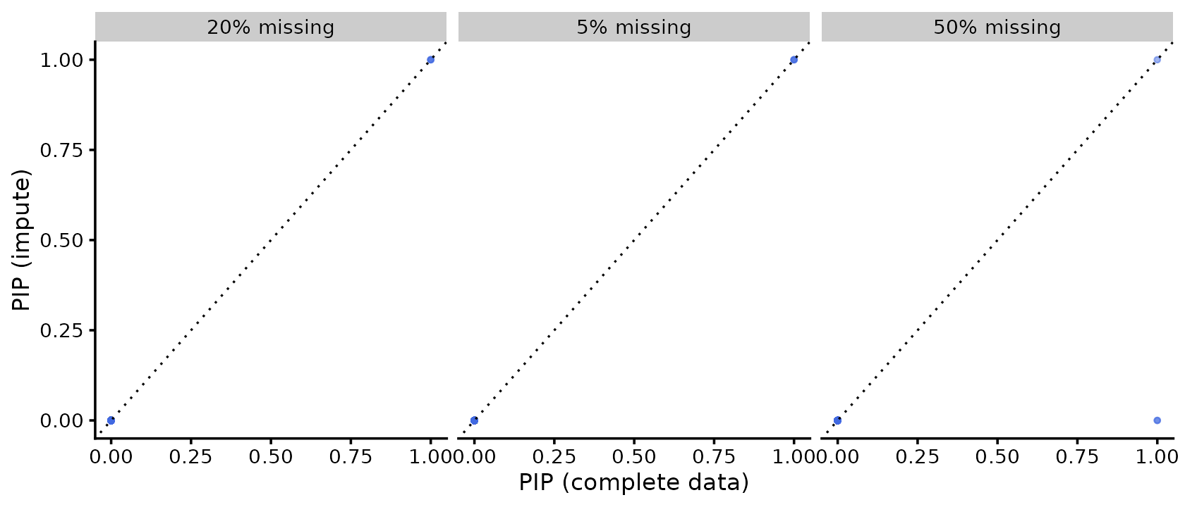
It performs well in terms of FDR but there is power loss particularly as missing rate goes higher.
Block missing data (cross-population scenario)
In a cross-population analysis, different cohorts may measure different subsets of traits. We simulate this by making the first 5 traits observed only in the first half of samples, and the last 5 traits only in the second half.
Y_block <- Y_complete
half <- n %/% 2
Y_block[1:half, 6:10] <- NA
Y_block[(half + 1):n, 1:5] <- NA
cat("Block missing pattern:\n")
cat("  Samples 1-", half, ": traits 1-5 observed, 6-10 missing\n")
cat("  Samples", half + 1, "-", n, ": traits 6-10 observed, 1-5 missing\n")
cat("  Total missing:", sum(is.na(Y_block)), "/", length(Y_block),
    sprintf("(%.0f%%)\n", 100 * mean(is.na(Y_block))))
# Block missing pattern:
#   Samples 1- 287 : traits 1-5 observed, 6-10 missing
#   Samples 288 - 574 : traits 6-10 observed, 1-5 missing
#   Total missing: 2870 / 5740 (50%)
The default "approximate" method handles this well:
fit_block <- mvsusie(X, Y_block, L = 10,
                     prior_variance = prior)
# mvsusie: N=574, J=1001, R=10, L=10 [mem: 0.20 GB]
# Warning: Cholesky failed for 10x10 matrix; falling back to SVD pseudo-inverse
# Residual variance set, common_cov=FALSE [mem: 0.25 GB]
# Prior: K=15 mixture components [mem: 0.25 GB]
# Eigendecomposition cache: K=15, common_cov=FALSE [mem: 0.28 GB]
# Model initialized: J=1001, R=10, L=10, K=15 [mem: 0.28 GB]
# iter          ELBO       delta   sigma2      mem      V
#    1    -4132.8494           -   diag[0.949,1.38]   0.28 GB  [1.36e-01, 4.68e-02, 2.71e-02, 0 x 7]
#    2    -4126.1604    6.69e+00   diag[0.949,1.38]   0.28 GB  [1.12e-01, 3.77e-02, 2.24e-02, 0 x 7]
#    3    -4126.1602    1.82e-04   diag[0.949,1.38]   0.28 GB  [1.12e-01, 3.77e-02, 2.24e-02, 0 x 7]
#    4    -4126.1602    7.13e-08   diag[0.949,1.38]   0.28 GB  [1.12e-01, 3.77e-02, 2.24e-02, 0 x 7]  converged
# Eigendecomposition cache: K=15, common_cov=FALSE [mem: 0.29 GB]
# Model initialized: J=1001, R=10, L=10, K=15 [mem: 0.29 GB]
# iter          ELBO       delta   sigma2      mem      V
#    1    -4099.9220           -   diag[0.856,1.14]   0.29 GB  [1.39e-01, 4.72e-02, 2.87e-02, 0 x 7]
#    2    -4093.3519    6.57e+00   diag[0.856,1.14]   0.29 GB  [1.16e-01, 3.91e-02, 2.37e-02, 0 x 7]
#    3    -4093.3518    6.17e-05   diag[0.856,1.14]   0.29 GB  [1.16e-01, 3.91e-02, 2.37e-02, 0 x 7]  converged
# Block ascent iter 1: ELBO=-4093.3518, change=32.81, sigma2=[0.964, 0.943, 0.961, 1.143, 0.977, 0.856, 0.942, 0.93, 1.112, 1.046]
# Eigendecomposition cache: K=15, common_cov=FALSE [mem: 0.29 GB]
# Model initialized: J=1001, R=10, L=10, K=15 [mem: 0.29 GB]
# iter          ELBO       delta   sigma2      mem      V
#    1    -4099.9092           -   diag[0.854,1.14]   0.29 GB  [1.39e-01, 4.72e-02, 2.88e-02, 0 x 7]
#    2    -4093.3390    6.57e+00   diag[0.854,1.14]   0.29 GB  [1.16e-01, 3.91e-02, 2.37e-02, 0 x 7]
#    3    -4093.3389    6.15e-05   diag[0.854,1.14]   0.29 GB  [1.16e-01, 3.91e-02, 2.37e-02, 0 x 7]  converged
# Block ascent iter 2: ELBO=-4093.3389, change=0.01293, sigma2=[0.962, 0.943, 0.959, 1.138, 0.976, 0.854, 0.937, 0.928, 1.111, 1.045]
# WARNING: "Cholesky failed for 10x10 matrix; falling back to SVD pseudo-inverse" occurred 15 times total (14 suppressed)
check_cs(fit_block, causal, "Block (approximate)")
# Block (approximate): 3 CS (3 true, 0 false), 3/4 causal captured
pdat <- data.frame(complete = fit_complete$pip,
                   block = fit_block$pip)
ggplot(pdat, aes(x = complete, y = block)) +
  geom_point(shape = 20, size = 1.5, color = "royalblue", alpha = 0.5) +
  geom_abline(intercept = 0, slope = 1, linetype = "dotted") +
  labs(x = "PIP (complete data)", y = "PIP (block missing)") +
  theme_cowplot(font_size = 12)
mvSuSiE borrows information across the observed portions to identify causal signals even when no single sample has all traits observed.
Why not use impute for block missing?
The "impute" method struggles with block-structured
missingness because traits from different blocks are never observed
together, making it impossible to impute correctly:
fit_block_imp <- mvsusie(X, Y_block, L = 10,
                         prior_variance = prior,
                         missing_y_method = "impute")
# mvsusie: N=574, J=1001, R=10, L=10 [mem: 0.21 GB]
# WARNING: Missingness is block-structured: 25 trait pair(s) are never jointly observed. Imputation cannot estimate cross-block covariances and will lose power. Consider using missing_y_method='approximate' or 'exact'.
# Residual variance set, common_cov=TRUE [mem: 0.21 GB]
# Prior: K=15 mixture components [mem: 0.21 GB]
# WARNING: Using PIP-based convergence (instead of ELBO) for impute method: the variational imputation does not guarantee a monotone ELBO, so PIP convergence is used as a stable alternative.
# Eigendecomposition cache: K=15, common_cov=TRUE [mem: 0.22 GB]
# Model initialized: J=1001, R=10, L=10, K=15 [mem: 0.22 GB]
# iter          ELBO       delta   sigma2      mem      V
#    1    -4205.5001           -   diag[0.949,1.38]   0.22 GB  [3.10e-02, 0 x 9]
# iter   2: max|d(alpha,PIP)|=2.96e-01, V=[5.50e-02, 0 x 9] [mem: 0.22 GB]
# iter   3: max|d(alpha,PIP)|=3.63e-01, V=[7.75e-02, 0 x 9] [mem: 0.22 GB]
# iter   4: max|d(alpha,PIP)|=3.64e-01, V=[9.28e-02, 0 x 9] [mem: 0.22 GB]
# iter   5: max|d(alpha,PIP)|=8.31e-06, V=[1.02e-01, 0 x 9] -- converged (alpha_pip_fixed_point) [mem: 0.22 GB]
check_cs(fit_block_imp, causal, "Block (impute)")
# Block (impute): 1 CS (1 true, 0 false), 1/4 causal captured
pdat <- data.frame(
  complete = rep(fit_complete$pip, 2),
  missing = c(fit_block$pip, fit_block_imp$pip),
  method = rep(c("approximate (default)", "impute"), each = p)
)
ggplot(pdat, aes(x = complete, y = missing)) +
  geom_point(shape = 20, size = 1.5, color = "royalblue", alpha = 0.5) +
  geom_abline(intercept = 0, slope = 1, linetype = "dotted") +
  facet_wrap(~method) +
  labs(x = "PIP (complete data)", y = "PIP (block missing)") +
  theme_cowplot(font_size = 10)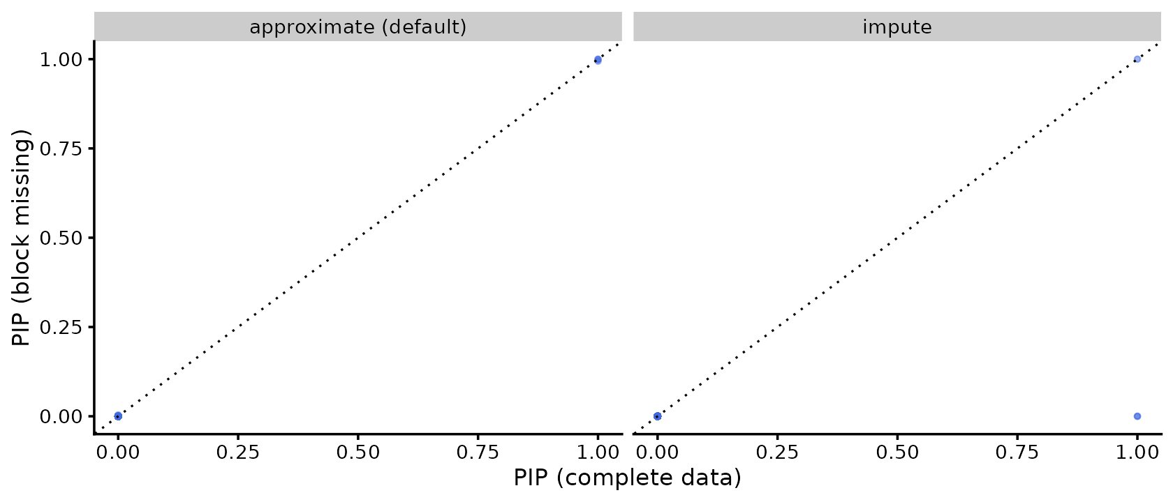
The "approximate" method recovers complete-data PIPs
well, while "impute" loses substantial power.
Missing data methods
mvSuSiE provides three methods for handling missing data, controlled
by the missing_y_method argument:
"approximate"(default): per-outcome centering with per-pattern residual variance correction. Fast and accurate; designed for the block-structured missingness common in multi-population analyses."exact": uses full residual covariance correction to account for intercepts. Produces similiar results to"approximate"at higher computational cost."impute": variational imputation that iteratively estimates missing values. Works well for scattered (MCAR) missing data at low missing rate but loses power for high or block-structured missingness.
fit_approx <- mvsusie(X, Y_miss_20, L = 10, prior_variance = prior,
                      estimate_prior_variance = TRUE,
                      missing_y_method = "approximate",
                      standardize = TRUE, verbose = FALSE)
fit_exact <- mvsusie(X, Y_miss_20, L = 10, prior_variance = prior,
                     estimate_prior_variance = TRUE,
                     missing_y_method = "exact",
                     standardize = TRUE, verbose = FALSE)

cat("20% MCAR:\n")
check_cs(fit_approx, causal, "  approximate")
check_cs(fit_exact, causal, "  exact")
cat("  PIP correlation (approx vs exact):", round(cor(fit_approx$pip, fit_exact$pip), 6), "\n")
# 20% MCAR:
#   approximate: 4 CS (4 true, 0 false), 4/4 causal captured
#   exact: 4 CS (4 true, 0 false), 4/4 causal captured
#   PIP correlation (approx vs exact): 1
For most applications, the default "approximate" method
provides a good balance of speed and accuracy.