Distinguishing linkage from pleiotropy
Gao Wang
2026-05-17
Source:vignettes/linkage_vs_pleiotropy.Rmd
linkage_vs_pleiotropy.RmdIn multi-trait fine-mapping it is possible in principle, though not always in practice, to distinguish between pleiotropy (one SNP affecting multiple traits) and linkage (different correlated SNPs each affecting different traits). When two correlated SNPs have distinct trait-specific effects, if the analysis is sufficiently powered, mvSuSiE can separate them into different credible sets, resolving LD-induced pleiotropy.
LD-induced pleiotropy: the problem
Consider two causal SNPs in negative LD (r \approx -0.66). SNP 1 affects traits 1–5 and SNP 2 affects traits 6–10. Because of the negative LD, the marginal association statistics show signal in all 10 traits for both SNPs, positive for the traits they truly affect and negative for the other traits (due to their “LD buddies”). This creates the appearance of broad pleiotropy when in reality each SNP is trait-specific.
data(simdata)
X <- simdata$raw$X
n <- nrow(X); p <- ncol(X); r <- 10

# Find a pair of SNPs with strong negative LD
R_mat <- cor(X)
pairs <- which(R_mat < -0.6 & R_mat > -0.8 &
               upper.tri(R_mat), arr.ind = TRUE)
snp1 <- pairs[1, 1]
snp2 <- pairs[1, 2]
cat(sprintf("Causal SNPs: %d and %d (LD r = %.3f)\n",
            snp1, snp2, R_mat[snp1, snp2]))
# Causal SNPs: 1 and 14 (LD r = -0.660)
We set per-trait PVE (heritability) at \approx 7\text{--}9\%, consistent with a moderately strong eQTL signal,
B <- matrix(0, p, r)
effect_size <- 2.0
B[snp1, 1:5] <- effect_size    # SNP 1 -> traits 1-5
B[snp2, 6:10] <- effect_size   # SNP 2 -> traits 6-10
Y <- X %*% B + matrix(rnorm(n * r), n, r)

# Per-trait PVE
pve <- sapply(1:r, function(t) {
  var(X %*% B[, t]) / var(Y[, t])
})
cat(sprintf("Per-trait PVE range: %.1f%% -- %.1f%%\n",
            100 * min(pve), 100 * max(pve)))
# Per-trait PVE range: 7.0% -- 9.0%
Marginal associations are misleading
The marginal z-scores and p-values show associations across almost all 10 traits for both SNPs, due to the negative LD confounding:
Z <- calc_z(X, Y, center = TRUE, scale = TRUE)
pval <- 2 * pnorm(-abs(Z))

z_dat <- data.frame(
  trait = rep(paste0("T", 1:r), 2),
  zscore = c(Z[snp1, ], Z[snp2, ]),
  pval = c(pval[snp1, ], pval[snp2, ]),
  snp = rep(c(paste("SNP", snp1), paste("SNP", snp2)), each = r)
)
z_dat$trait <- factor(z_dat$trait, levels = paste0("T", 1:r))
z_dat$direction <- factor(ifelse(z_dat$zscore > 0, "+1", "-1"),
                          levels = c("-1", "+1"))
z_dat$logp <- -log10(z_dat$pval)

ggplot(z_dat, aes(x = snp, y = trait, fill = direction, size = logp)) +
  geom_point(shape = 21, stroke = 0.5, color = "white") +
  scale_fill_manual(values = c("darkblue", "red"), drop = FALSE) +
  scale_size(range = c(1, 6),
             breaks = unname(round(quantile(z_dat$logp,
                                            seq(0, 1, length.out = 4)), 1))) +
  labs(x = "", y = "", fill = "direction", size = expression(-log[10](p))) +
  guides(fill = guide_legend(override.aes = list(size = 2)),
         size = guide_legend(override.aes = list(shape = 21, fill = "black",
                                                  color = "white",
                                                  stroke = 0.5))) +
  theme_cowplot(font_size = 10) +
  background_grid(major = "xy", minor = "none",
                  size.major = 0.3, colour.major = "grey85") +
  panel_border(colour = "grey70") +
  theme(axis.text.x = element_text(angle = 45, hjust = 1))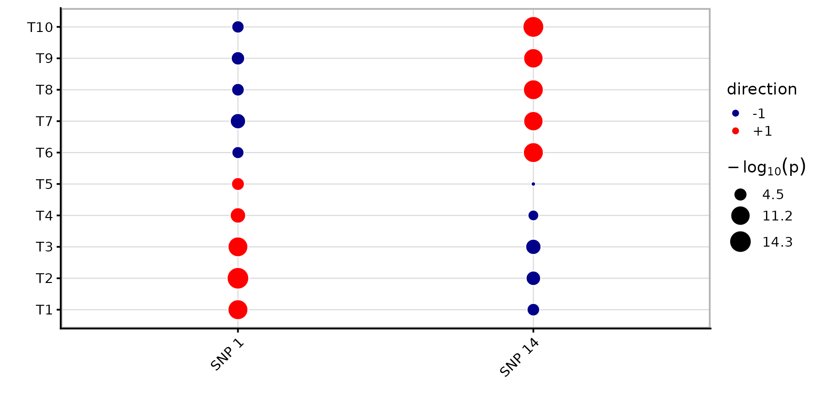
Both SNPs show significant associations in most of the 10 traits. All of them have p<0.05. Without multi-trait fine-mapping, one might conclude that both SNPs are broadly pleiotropic, with positive effects in 5 traits and negative in the other 5.
Resolving with mvSuSiE
mvSuSiE with a mixture prior can separate the two linked signals into different credible sets, each with its own trait-specific effect pattern.
prior <- create_mixture_prior(R = r)
fit <- mvsusie(X, Y, L = 10,
               prior_variance = prior)
# mvsusie: N=574, J=1001, R=10, L=10 [mem: 0.19 GB]
# Residual variance set, common_cov=TRUE [mem: 0.19 GB]
# Prior: K=15 mixture components [mem: 0.19 GB]
# Eigendecomposition cache: K=15, common_cov=TRUE [mem: 0.19 GB]
# Model initialized: J=1001, R=10, L=10, K=15 [mem: 0.19 GB]
# iter          ELBO       delta   sigma2      mem      V
#    1    -8163.9461           -   diag[0.911,1.17]   0.20 GB  [7.11e-02, 1.01e-02, 0 x 8]
#    2    -8116.8842    4.71e+01   diag[0.843,1.12]   0.20 GB  [6.09e-02, 1.73e-02, 0 x 8]
#    3    -8111.5062    5.38e+00   diag[0.842,1.11]   0.20 GB  [4.97e-02, 2.40e-02, 0 x 8]
#    4    -8110.3537    1.15e+00   diag[0.842,1.11]   0.20 GB  [4.49e-02, 2.75e-02, 0 x 8]
#    5    -8109.6771    6.77e-01   diag[0.842,1.11]   0.20 GB  [5.64e-02, 3.77e-02, 0 x 8]
#    6    -8109.6056    7.15e-02   diag[0.842,1.1]   0.20 GB  [5.51e-02, 3.87e-02, 0 x 8]
#    7    -8109.5910    1.45e-02   diag[0.842,1.1]   0.20 GB  [5.45e-02, 3.92e-02, 0 x 8]
#    8    -8109.5880    2.99e-03   diag[0.842,1.1]   0.20 GB  [5.42e-02, 3.94e-02, 0 x 8]
#    9    -8109.5874    6.21e-04   diag[0.842,1.1]   0.20 GB  [5.40e-02, 3.95e-02, 0 x 8]
#   10    -8109.5873    1.30e-04   diag[0.842,1.1]   0.20 GB  [5.39e-02, 3.96e-02, 0 x 8]
#   11    -8109.5873    2.77e-05   diag[0.842,1.1]   0.20 GB  [5.39e-02, 3.96e-02, 0 x 8]  converged
cat("Number of credible sets:", length(fit$sets$cs), "\n\n")
for (cs_name in names(fit$sets$cs)) {
  cs_vars <- fit$sets$cs[[cs_name]]
  l_idx <- as.integer(gsub("L", "", cs_name))
  sig_traits <- which(fit$single_effect_lfsr[l_idx, ] < 0.01)
  has_snp1 <- snp1 %in% cs_vars
  has_snp2 <- snp2 %in% cs_vars
  cat(sprintf("%s: %d SNP(s), contains SNP%d=%s SNP%d=%s\n",
              cs_name, length(cs_vars),
              snp1, has_snp1, snp2, has_snp2))
  cat(sprintf("  Significant traits (lfsr < 0.01): %s\n",
              paste(sig_traits, collapse = ", ")))
}
# Number of credible sets: 2
#
# L1: 1 SNP(s), contains SNP1=FALSE SNP14=TRUE
#   Significant traits (lfsr < 0.01): 6, 7, 8, 9, 10
# L2: 1 SNP(s), contains SNP1=TRUE SNP14=FALSE
#   Significant traits (lfsr < 0.01): 1, 2, 3, 4, 5
Two CS are identified,
out <- mvsusie_plot(fit, add_cs = TRUE, lfsr_cutoff = 0.05)
out$pip_plot
Effect plot (mvSuSiE)
The mvsusie_plot effect plot shows that each credible
set has effects in only its 5 causal traits, which looks different from
the marginal association plots previously shown.
out$effect_plot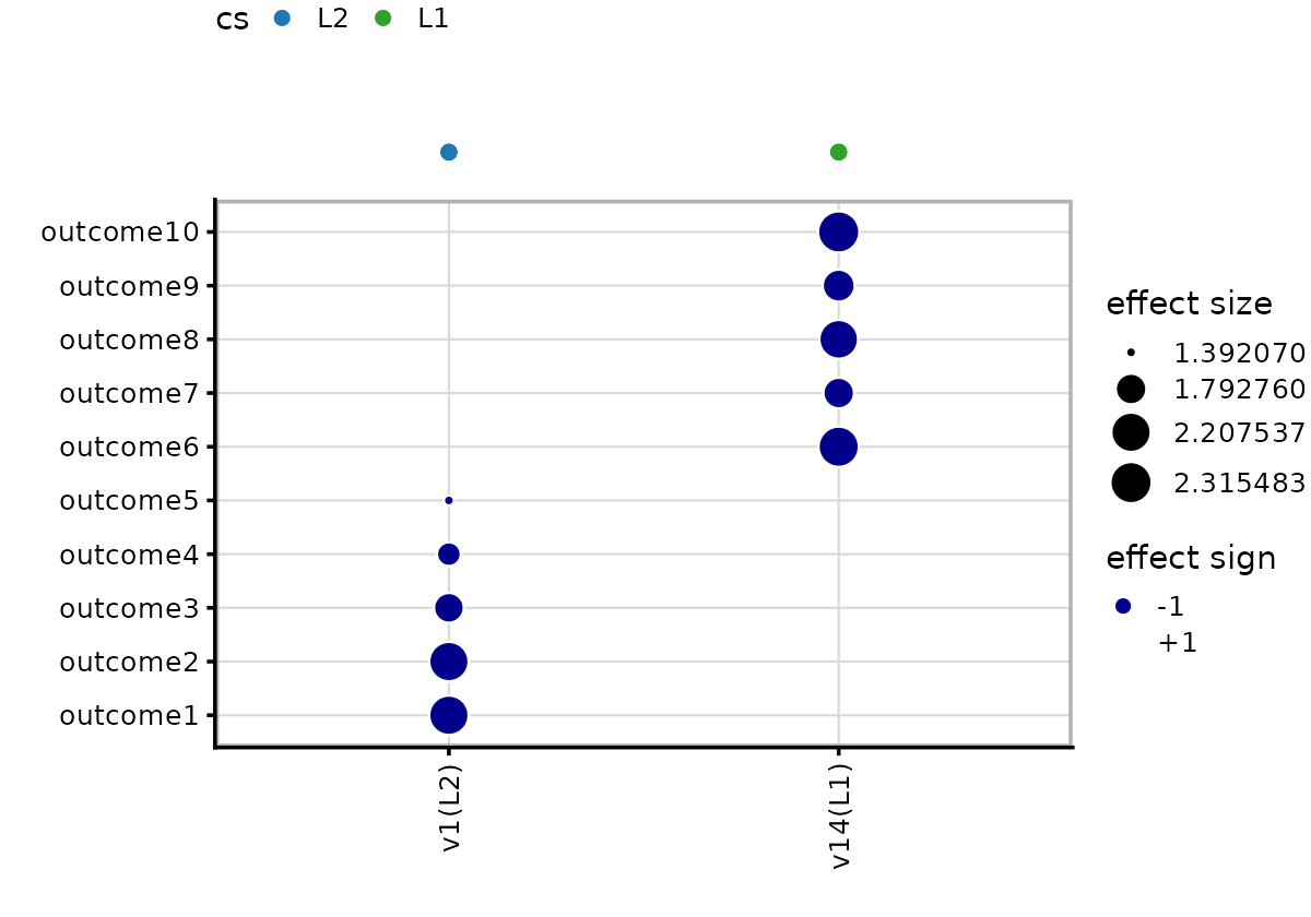
Marginal z-scores for CS variants
For comparison, we plot the marginal z-scores for the same variants that appear in the mvSuSiE credible sets.
# Extract CS SNPs and their z-scores
cs_z_dat <- data.frame()
for (cs_name in names(fit$sets$cs)) {
  cs_vars <- fit$sets$cs[[cs_name]]
  for (j in cs_vars) {
    df <- data.frame(
      trait = paste0("T", 1:r),
      zscore = Z[j, ],
      pval = pval[j, ],
      snp_cs = paste0("SNP", j, "(", cs_name, ")"),
      cs = cs_name,
      stringsAsFactors = FALSE
    )
    cs_z_dat <- rbind(cs_z_dat, df)
  }
}
cs_z_dat$trait <- factor(cs_z_dat$trait, levels = paste0("T", 1:r))
cs_z_dat$direction <- factor(ifelse(cs_z_dat$zscore > 0, "+1", "-1"),
                             levels = c("-1", "+1"))
cs_z_dat$logp <- -log10(cs_z_dat$pval)

ggplot(cs_z_dat, aes(x = snp_cs, y = trait,
                     fill = direction, size = logp)) +
  geom_point(shape = 21, stroke = 0.5, color = "white") +
  scale_fill_manual(values = c("darkblue", "red"), drop = FALSE) +
  scale_size(range = c(1, 6),
             breaks = unname(round(quantile(cs_z_dat$logp,
                                            seq(0, 1, length.out = 4)), 1))) +
  labs(x = "", y = "", fill = "direction",
       size = expression(-log[10](p)),
       title = "Marginal z-scores") +
  guides(fill = guide_legend(override.aes = list(size = 2)),
         size = guide_legend(override.aes = list(shape = 21, fill = "black",
                                                  color = "white",
                                                  stroke = 0.5))) +
  theme_cowplot(font_size = 10) +
  background_grid(major = "xy", minor = "none",
                  size.major = 0.3, colour.major = "grey85") +
  panel_border(colour = "grey70") +
  theme(axis.text.x = element_text(angle = 45, hjust = 1))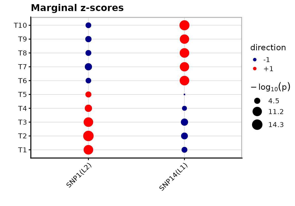
Comparison with univariate fine-mapping
Here we analyze 10 traits seperately using susie():
for (t in c(1:10)) {
  fit_uv <- susie(X, Y[, t], L = 10, standardize = TRUE)
  if (length(fit_uv$sets$cs) > 0) {
    cs1 <- fit_uv$sets$cs[[1]]
    cat(sprintf("Trait %d CS: %d SNPs, contains SNP%d=%s, SNP%d=%s\n",
                t, length(cs1),
                snp1, snp1 %in% cs1,
                snp2, snp2 %in% cs1))
  } else {
    cat(sprintf("Trait %d: no CS found\n", t))
  }
}
# Trait 1 CS: 1 SNPs, contains SNP1=TRUE, SNP14=FALSE
# Trait 2 CS: 1 SNPs, contains SNP1=TRUE, SNP14=FALSE
# Trait 3 CS: 1 SNPs, contains SNP1=TRUE, SNP14=FALSE
# Trait 4 CS: 2 SNPs, contains SNP1=TRUE, SNP14=FALSE
# Trait 5: no CS found
# Trait 6 CS: 1 SNPs, contains SNP1=FALSE, SNP14=TRUE
# Trait 7 CS: 2 SNPs, contains SNP1=FALSE, SNP14=TRUE
# Trait 8 CS: 1 SNPs, contains SNP1=FALSE, SNP14=TRUE
# Trait 9 CS: 1 SNPs, contains SNP1=FALSE, SNP14=TRUE
# Trait 10 CS: 1 SNPs, contains SNP1=FALSE, SNP14=TRUE
The challenge of weak LD contrast
When the effects are smaller relative to noise, both univariate and multivariate methods lose power. With PVE around 2–3%, mvSuSiE may find fewer credible sets or may not fully resolve the two signals.
set.seed(2)
B_weak <- matrix(0, p, r)
B_weak[snp1, 1:5] <- 1.0
B_weak[snp2, 6:10] <- 1.0
Y_weak <- X %*% B_weak + matrix(rnorm(n * r), n, r)

pve_weak <- sapply(1:r, function(t) {
  var(X %*% B_weak[, t]) / var(Y_weak[, t])
})
cat(sprintf("Per-trait PVE range: %.1f%% -- %.1f%%\n",
            100 * min(pve_weak), 100 * max(pve_weak)))

fit_weak <- mvsusie(X, Y_weak, L = 10,
                    prior_variance = prior)
# mvsusie: N=574, J=1001, R=10, L=10 [mem: 0.20 GB]
# Residual variance set, common_cov=TRUE [mem: 0.20 GB]
# Prior: K=15 mixture components [mem: 0.20 GB]
# Eigendecomposition cache: K=15, common_cov=TRUE [mem: 0.21 GB]
# Model initialized: J=1001, R=10, L=10, K=15 [mem: 0.21 GB]
# iter          ELBO       delta   sigma2      mem      V
#    1    -8101.2876           -   diag[0.856,1.11]   0.21 GB  [1.66e-02, 0 x 9]
#    2    -8096.6949    4.59e+00   diag[0.846,1.11]   0.21 GB  [1.42e-02, 0 x 9]
#    3    -8096.6907    4.17e-03   diag[0.847,1.11]   0.21 GB  [1.42e-02, 0 x 9]
#    4    -8096.6905    1.95e-04   diag[0.847,1.11]   0.21 GB  [1.42e-02, 0 x 9]
#    5    -8096.6905    9.49e-06   diag[0.847,1.11]   0.21 GB  [1.42e-02, 0 x 9]  converged
out <- mvsusie_plot(fit_weak, add_cs = TRUE, lfsr_cutoff = 0.05)
out$pip_plot
out$effect_plot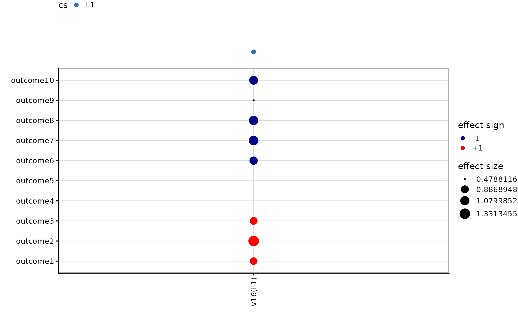
# Per-trait PVE range: 1.8% -- 2.4%