Scaling mvSuSiE to many traits

This vignette demonstrates running mvSuSiE with a relatively large number of traits (R = 100) and provides benchmark timings for typical configurations.

library(mvsusieR)
library(ggplot2)
library(cowplot)

Key considerations for large R

When the number of traits R is large (e.g., R > 50):

Prior specification: A canonical or data-driven mixture prior is recommended. For very large R, the number of canonical prior matrices grows, so data-driven priors from mashr that select only the relevant components are preferred.
Precompute cache: Setting precompute_cache = TRUE (default) caches eigendecompositions of the prior covariance matrices, providing substantial speedups for large R. The trade-off is increased memory usage.
Residual variance estimation: When N < R, the sample covariance of Y is singular. In this case, regularization methods such as using flashier package can be used to estimate a low-rank plus diagonal residual covariance, and specified into mvSuSiE via residual_variance = .... If still left to NULL, mvsusie uses pairwise complete covariance estimation with a positive definiteness correction as the initial residual covariance.
C++ acceleration: The core computations are implemented in Rcpp for efficiency and is available by default. Multi-threading is available via the n_thread argument.

Example: R = 100

data(simdata)
X <- simdata$raw$X
n <- nrow(X); p <- ncol(X); r <- 100

# Simulate 100 traits with shared causal variants
set.seed(42)
B <- matrix(0, p, r)
causal <- sort(sample(p, 4))
for (j in causal) B[j, ] <- rnorm(r, 0, 0.3)
Y <- X %*% B + matrix(rnorm(n * r), n, r)
cat(sprintf("Data: %d samples, %d SNPs, %d traits\n", n, p, r))
cat("Causal SNPs:", causal, "\n")

# Canonical prior (105 components for R=100)
prior <- create_mixture_prior(R = r)
cat("Prior components:", prior$n_component, "\n")
# Data: 574 samples, 1001 SNPs, 100 traits
# Causal SNPs: 153 321 561 997 
# Prior components:

t0 <- proc.time()
fit <- mvsusie(X, Y, L = 10,
               prior_variance = prior)
# mvsusie: N=574, J=1001, R=100, L=10 [mem: 0.18 GB]
# Residual variance set, common_cov=TRUE [mem: 0.18 GB]
# Prior: K=105 mixture components [mem: 0.18 GB]
# Eigendecomposition cache: K=105, common_cov=TRUE [mem: 0.23 GB]
# Model initialized: J=1001, R=100, L=10, K=105 [mem: 0.23 GB]
# iter          ELBO       delta   sigma2      mem      V
#    1   -79941.5755           -   diag[0.878,1.29]   0.24 GB  [1.78e-02, 1.02e-02, 9.53e-03, 0 x 7]
#    2   -79517.5651    4.24e+02   diag[0.865,1.16]   0.24 GB  [2.87e-02, 1.64e-02, 1.75e-02, 0 x 7]
#    3   -79485.3156    3.22e+01   diag[0.863,1.16]   0.24 GB  [2.98e-02, 1.76e-02, 1.88e-02, 0 x 7]
#    4   -79484.9738    3.42e-01   diag[0.863,1.16]   0.24 GB  [2.99e-02, 1.77e-02, 1.89e-02, 0 x 7]
#    5   -79484.9677    6.06e-03   diag[0.863,1.16]   0.24 GB  [2.99e-02, 1.77e-02, 1.89e-02, 0 x 7]
#    6   -79484.9676    1.33e-04   diag[0.863,1.16]   0.24 GB  [2.99e-02, 1.77e-02, 1.89e-02, 0 x 7]
#    7   -79484.9676    4.18e-06   diag[0.863,1.16]   0.24 GB  [2.99e-02, 1.77e-02, 1.89e-02, 0 x 7]  converged
timing <- (proc.time() - t0)[["elapsed"]]
cat(sprintf("Elapsed time: %.1f seconds\n", timing))
cat(sprintf("IBSS iterations: %d\n", length(fit$elbo)))
cat(sprintf("Credible sets: %d\n", length(fit$sets$cs)))
# Elapsed time: 45.7 seconds
# IBSS iterations: 7
# Credible sets: 3

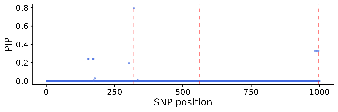
# Check which causal SNPs are captured
for (cs_name in names(fit$sets$cs)) {
  cs_vars <- fit$sets$cs[[cs_name]]
  captured <- intersect(cs_vars, causal)
  cat(sprintf("%s: %d SNPs, captures causal %s\n",
              cs_name, length(cs_vars),
              if (length(captured) > 0) paste(captured, collapse = ", ")
              else "none"))
}
# L2: 4 SNPs, captures causal 153
# L1: 3 SNPs, captures causal 997
# L3: 2 SNPs, captures causal 321

pdat <- data.frame(pos = seq_len(p), pip = fit$pip)
ggplot(pdat, aes(x = pos, y = pip)) +
  geom_point(shape = 20, size = 1, color = "royalblue", alpha = 0.5) +
  geom_vline(xintercept = causal, linetype = "dashed",
             color = "red", alpha = 0.5) +
  labs(x = "SNP position", y = "PIP") +
  theme_cowplot(font_size = 12)

Gao Wang

2026-05-17

Key considerations for large R

Example: R = 100