Input data formats for mvSuSiE
Gao Wang
2026-05-17
Source:vignettes/input_data_format.Rmd
input_data_format.RmdmvSuSiE provides three interfaces for fitting multivariate Sum of Single Effects models, depending on the type of data available:
mvsusie(): individual-level data (genotype matrix X and phenotype matrix Y).mvsusie_ss(): sufficient statistics (X^TX, X^TY, Y^TY and the sample size N).mvsusie_rss(): summary statistics (z-scores and an LD matrix, or effect estimates and standard errors).
This vignette demonstrates all three interfaces on the same data set,
verifies equivalence, and examines the z-score-only path where the
outcome covariance varY is not available.
Simulate data
We use realistic genotypes and simulate a phenotype matrix with R = 10 traits.
data(simdata)
X <- simdata$raw$X
n <- nrow(X)
p <- ncol(X)
r <- 10
cat(sprintf("Genotype matrix: %d samples x %d SNPs\n", n, p))

causal <- sort(sample(p, 4))
B <- matrix(0, p, r)
for (j in causal) B[j, ] <- rnorm(r, 0, 0.5)
Y <- X %*% B + matrix(rnorm(n * r), n, r)
cat(sprintf("Phenotype matrix: %d samples x %d traits\n", n, r))
cat("Causal SNPs:", causal, "\n")
# Genotype matrix: 574 samples x 1001 SNPs
# Phenotype matrix: 574 samples x 10 traits
# Causal SNPs: 129 679 836 930
prior <- create_mixture_prior(R = r)
resid_var <- diag(r)
Interface 1 and 2: Individual-level and sufficient statistics
We fit both interfaces with their defaults
(estimate_residual_variance = TRUE).
fit <- mvsusie(X, Y, L = 10,
               prior_variance = prior,
               residual_variance = resid_var,
               estimate_prior_variance = TRUE,
               standardize = TRUE)
# mvsusie: N=574, J=1001, R=10, L=10 [mem: 0.16 GB]
# Residual variance set, common_cov=TRUE [mem: 0.17 GB]
# Prior: K=15 mixture components [mem: 0.17 GB]
# Eigendecomposition cache: K=15, common_cov=TRUE [mem: 0.17 GB]
# Model initialized: J=1001, R=10, L=10, K=15 [mem: 0.17 GB]
# iter          ELBO       delta   sigma2      mem      V
#    1    -8217.4864           -   diag[1,1]   0.17 GB  [1.53e-01, 3.95e-02, 2.49e-02, 0 x 7]
#    2    -8185.3051    3.22e+01   diag[0.862,1.09]   0.17 GB  [1.28e-01, 3.29e-02, 2.05e-02, 0 x 7]
#    3    -8185.3033    1.75e-03   diag[0.861,1.09]   0.17 GB  [1.28e-01, 3.29e-02, 2.05e-02, 0 x 7]
#    4    -8185.3033    1.53e-07   diag[0.861,1.09]   0.17 GB  [1.28e-01, 3.29e-02, 2.05e-02, 0 x 7]  converged
X_colmeans <- colMeans(X)
Y_colmeans <- colMeans(Y)
Xc <- scale(X, center = TRUE, scale = FALSE)
Yc <- scale(Y, center = TRUE, scale = FALSE)
XtX <- crossprod(Xc)
XtY <- crossprod(Xc, Yc)
YtY <- crossprod(Yc)
fit_ss <- mvsusie_ss(XtX, XtY, YtY, N = n, L = 10,
                     X_colmeans = X_colmeans,
                     Y_colmeans = Y_colmeans,
                     prior_variance = prior,
                     residual_variance = resid_var,
                     estimate_prior_variance = TRUE,
                     standardize = TRUE)
# Eigendecomposition cache: K=15, common_cov=TRUE [mem: 0.19 GB]
# Model initialized: J=1001, R=10, L=10, K=15 [mem: 0.19 GB]
# iter          ELBO       delta   sigma2      mem      V
#    1    -8217.4864           -   diag[1,1]   0.19 GB  [1.53e-01, 3.95e-02, 2.49e-02, 0 x 7]
#    2    -8185.3051    3.22e+01   diag[0.862,1.09]   0.19 GB  [1.28e-01, 3.29e-02, 2.05e-02, 0 x 7]
#    3    -8185.3033    1.75e-03   diag[0.861,1.09]   0.19 GB  [1.28e-01, 3.29e-02, 2.05e-02, 0 x 7]
#    4    -8185.3033    1.53e-07   diag[0.861,1.09]   0.19 GB  [1.28e-01, 3.29e-02, 2.05e-02, 0 x 7]  converged
# WARNING: Xcorr is not symmetric; using (Xcorr + t(Xcorr))/2.
cat("mvsusie vs mvsusie_ss (both defaults):\n")
cat("  max |PIP diff|:", max(abs(fit$pip - fit_ss$pip)), "\n")
cat("  max |coef diff|:", max(abs(coef(fit)[-1, ] - coef(fit_ss)[-1, ])), "\n")
# mvsusie vs mvsusie_ss (both defaults):
#   max |PIP diff|: 4.440892e-16
#   max |coef diff|: 3.590905e-12
The PIP and coefficient differences are at machine precision,
confirming that mvsusie() and mvsusie_ss() are
numerically identical when given the same data.
Interface 3a: RSS with full information
When effect estimates (Bhat), standard errors
(Shat), and the sample covariance of Y (varY)
are all provided alongside the LD matrix and sample size,
mvsusie_rss() reconstructs the exact sufficient statistics
and produces results identical to mvsusie() and
mvsusie_ss().
Bhat <- matrix(0, p, r)
Shat <- matrix(0, p, r)
for (outcome in seq_len(r)) {
  reg <- susieR:::univariate_regression(Xc, Yc[, outcome])
  Bhat[, outcome] <- reg$betahat
  Shat[, outcome] <- reg$sebetahat
}
LD <- cor(X)
varY_mat <- cov(Y)
fit_rss_bhat <- mvsusie_rss(Bhat = Bhat, Shat = Shat, R = LD,
                             N = n, varY = varY_mat, L = 10,
                             prior_variance = prior,
                             residual_variance = resid_var,
                             estimate_residual_variance = TRUE,
                             estimate_prior_variance = TRUE)
# Eigendecomposition cache: K=15, common_cov=TRUE [mem: 0.22 GB]
# Model initialized: J=1001, R=10, L=10, K=15 [mem: 0.22 GB]
# iter          ELBO       delta   sigma2      mem      V
#    1    -8217.4864           -   diag[1,1]   0.22 GB  [1.53e-01, 3.95e-02, 2.49e-02, 0 x 7]
#    2    -8185.3051    3.22e+01   diag[0.862,1.09]   0.22 GB  [1.28e-01, 3.29e-02, 2.05e-02, 0 x 7]
#    3    -8185.3033    1.75e-03   diag[0.861,1.09]   0.22 GB  [1.28e-01, 3.29e-02, 2.05e-02, 0 x 7]
#    4    -8185.3033    1.53e-07   diag[0.861,1.09]   0.22 GB  [1.28e-01, 3.29e-02, 2.05e-02, 0 x 7]  converged
# WARNING: Xcorr is not symmetric; using (Xcorr + t(Xcorr))/2.
cat("mvsusie vs mvsusie_rss (Bhat/Shat/varY):\n")
cat("  max |PIP diff|:", max(abs(fit$pip - fit_rss_bhat$pip)), "\n")
cat("  max |coef diff|:", max(abs(coef(fit)[-1, ] - coef(fit_rss_bhat)[-1, ])), "\n")
# mvsusie vs mvsusie_rss (Bhat/Shat/varY):
#   max |PIP diff|: 2.187139e-14
#   max |coef diff|: 1.092258e-09
With Bhat, Shat, and varY all
provided, mvsusie_rss() reconstructs the exact sufficient
statistics internally, so the PIPs and coefficients match
mvsusie() to machine precision.
Similarly, when z-scores are provided together with
varY, the PIPs also match closely. (The coefficients are on
a standardized scale in this case, so only PIPs are compared.)
Z <- calc_z(X, Y, center = TRUE, scale = TRUE)
fit_rss_zv <- mvsusie_rss(Z, LD, N = n, varY = varY_mat, L = 10,
                           prior_variance = prior,
                           residual_variance = resid_var,
                           estimate_residual_variance = TRUE,
                           estimate_prior_variance = TRUE)
# Eigendecomposition cache: K=15, common_cov=TRUE [mem: 0.22 GB]
# Model initialized: J=1001, R=10, L=10, K=15 [mem: 0.22 GB]
# iter          ELBO       delta   sigma2      mem      V
#    1    -7867.2783           -   diag[1,1]   0.22 GB  [1.01e-01, 2.62e-02, 1.64e-02, 0 x 7]
#    2    -7805.7980    6.15e+01   diag[0.678,0.992]   0.22 GB  [8.50e-02, 2.19e-02, 1.36e-02, 0 x 7]
#    3    -7805.7941    3.96e-03   diag[0.676,0.992]   0.22 GB  [8.51e-02, 2.19e-02, 1.36e-02, 0 x 7]
#    4    -7805.7941    2.63e-07   diag[0.676,0.992]   0.22 GB  [8.51e-02, 2.19e-02, 1.36e-02, 0 x 7]  converged
cat("mvsusie vs mvsusie_rss (Z + varY):\n")
cat("  max |PIP diff|:", max(abs(fit$pip - fit_rss_zv$pip)), "\n")
# mvsusie vs mvsusie_rss (Z + varY):
#   max |PIP diff|: 6.821876e-12
The z-score path with varY also produces PIPs that match
at near machine precision. The coefficients from this path are on a
standardized scale (see the coefficient section below), so only PIP
agreement is checked here.
Interface 3b: RSS with z-scores only (no varY)
In the most common summary-data scenario, only z-scores, the LD
matrix, and sample size are available — without varY or
Bhat/Shat. In this setting, the outcome
correlation cor(Y) needed for the Y^TY matrix is estimated internally from
near-null z-scores (SNPs with \max|Z| <
2). This estimate captures the residual correlation structure but
may miss signal-induced cross-trait correlations.
The default for this path is
estimate_residual_variance = FALSE, following the
recommendation in Zou et al.
(2022) that the residual variance is difficult to estimate reliably
from summary statistics alone.
fit_rss_f <- mvsusie_rss(Z, LD, N = n, L = 10,
                          prior_variance = prior,
                          residual_variance = resid_var,
                          estimate_residual_variance = FALSE,
                          estimate_prior_variance = TRUE)
# Eigendecomposition cache: K=15, common_cov=TRUE [mem: 0.22 GB]
# Model initialized: J=1001, R=10, L=10, K=15 [mem: 0.22 GB]
# iter          ELBO       delta   sigma2      mem      V
#    1    -7867.2783           -   diag[1,1]   0.23 GB  [1.01e-01, 2.62e-02, 1.64e-02, 0 x 7]
#    2    -7860.8696    6.41e+00   diag[1,1]   0.23 GB  [8.44e-02, 2.16e-02, 1.34e-02, 0 x 7]
#    3    -7860.8695    1.52e-04   diag[1,1]   0.23 GB  [8.44e-02, 2.16e-02, 1.34e-02, 0 x 7]
#    4    -7860.8695    1.92e-09   diag[1,1]   0.23 GB  [8.44e-02, 2.16e-02, 1.34e-02, 0 x 7]  converged
fit_rss_t <- mvsusie_rss(Z, LD, N = n, L = 10,
                          prior_variance = prior,
                          residual_variance = resid_var,
                          estimate_residual_variance = TRUE,
                          estimate_prior_variance = TRUE)
# WARNING: Estimating residual variance from summary statistics without providing varY may be inaccurate. Consider providing varY or setting estimate_residual_variance = FALSE.
# Eigendecomposition cache: K=15, common_cov=TRUE [mem: 0.23 GB]
# Model initialized: J=1001, R=10, L=10, K=15 [mem: 0.23 GB]
# iter          ELBO       delta   sigma2      mem      V
#    1    -7867.2783           -   diag[1,1]   0.23 GB  [1.01e-01, 2.62e-02, 1.64e-02, 0 x 7]
#    2    -7440.9957    4.26e+02   diag[0.678,0.992]   0.23 GB  [8.33e-02, 2.19e-02, 1.30e-02, 2.22e-03, 9.06e-04, 5.18e-04, 0 x 4]
#    3    -7440.1721    8.24e-01   diag[0.672,0.99]   0.23 GB  [8.39e-02, 2.20e-02, 1.31e-02, 2.32e-03, 1.31e-03, 6.75e-04, 4.69e-04, 0 x 3]
#    4    -7439.5917    5.80e-01   diag[0.671,0.989]   0.23 GB  [8.67e-02, 2.27e-02, 1.35e-02, 2.43e-03, 1.58e-03, 7.03e-04, 5.90e-04, 4.23e-04, 2.95e-04, 0 x 1]
#    5    -7439.2465    3.45e-01   diag[0.669,0.989]   0.23 GB  [9.09e-02, 2.36e-02, 1.40e-02, 2.47e-03, 1.66e-03, 6.57e-04, 5.84e-04, 5.03e-04, 4.25e-04, 3.04e-04]
#    6    -7439.1108    1.36e-01   diag[0.668,0.989]   0.23 GB  [9.37e-02, 2.41e-02, 1.41e-02, 2.47e-03, 1.82e-03, 6.39e-04, 5.83e-04, 5.26e-04, 4.72e-04, 4.05e-04]
#    7    -7439.0161    9.47e-02   diag[0.668,0.989]   0.23 GB  [9.35e-02, 2.41e-02, 1.41e-02, 2.48e-03, 2.04e-03, 6.76e-04, 6.07e-04, 5.57e-04, 5.12e-04, 4.64e-04]
#    8    -7438.9474    6.88e-02   diag[0.668,0.989]   0.23 GB  [9.21e-02, 2.38e-02, 1.39e-02, 2.50e-03, 2.18e-03, 7.01e-04, 6.25e-04, 5.83e-04, 5.45e-04, 5.07e-04]
#    9    -7438.9193    2.80e-02   diag[0.668,0.989]   0.23 GB  [9.09e-02, 2.35e-02, 1.38e-02, 2.52e-03, 2.25e-03, 6.83e-04, 6.35e-04, 6.01e-04, 5.69e-04, 5.37e-04]
#   10    -7438.9120    7.34e-03   diag[0.668,0.989]   0.23 GB  [9.01e-02, 2.33e-02, 1.38e-02, 2.53e-03, 2.27e-03, 6.47e-04, 6.39e-04, 6.12e-04, 5.85e-04, 5.58e-04]
#   11    -7438.9102    1.81e-03   diag[0.668,0.989]   0.23 GB  [8.98e-02, 2.32e-02, 1.37e-02, 2.54e-03, 2.28e-03, 6.18e-04, 6.34e-04, 6.19e-04, 5.96e-04, 5.73e-04]
#   12    -7438.9097    4.99e-04   diag[0.668,0.989]   0.23 GB  [8.97e-02, 2.32e-02, 1.37e-02, 2.54e-03, 2.28e-03, 6.01e-04, 6.25e-04, 6.21e-04, 6.04e-04, 5.84e-04]
#   13    -7438.9095    1.76e-04   diag[0.668,0.989]   0.23 GB  [8.96e-02, 2.32e-02, 1.37e-02, 2.54e-03, 2.28e-03, 5.94e-04, 6.15e-04, 6.19e-04, 6.09e-04, 5.93e-04]
#   14    -7438.9094    7.74e-05   diag[0.668,0.989]   0.23 GB  [8.96e-02, 2.32e-02, 1.37e-02, 2.54e-03, 2.28e-03, 5.92e-04, 6.07e-04, 6.15e-04, 6.11e-04, 5.99e-04]  converged
cat("=== Z-score only: FALSE vs TRUE ===\n")
cat("  Credible sets (FALSE):", length(fit_rss_f$sets$cs), "\n")
cat("  Credible sets (TRUE):", length(fit_rss_t$sets$cs), "\n")
cat("  PIP correlation:", round(cor(fit_rss_f$pip, fit_rss_t$pip), 4), "\n\n")

cat("=== Z-score only vs individual-level (defaults) ===\n")
cat("mvsusie (TRUE) vs mvsusie_rss z-only (FALSE):\n")
cat("  max |PIP diff|:", round(max(abs(fit$pip - fit_rss_f$pip)), 4), "\n")
cat("  PIP correlation:", round(cor(fit$pip, fit_rss_f$pip), 4), "\n\n")

cat("mvsusie (TRUE) vs mvsusie_rss z-only (TRUE):\n")
cat("  max |PIP diff|:", round(max(abs(fit$pip - fit_rss_t$pip)), 4), "\n")
cat("  PIP correlation:", round(cor(fit$pip, fit_rss_t$pip), 4), "\n\n")

cat("=== Z-score only vs Z + varY (both TRUE) ===\n")
cat("  max |PIP diff|:", round(max(abs(fit_rss_zv$pip - fit_rss_t$pip)), 4), "\n")
cat("  PIP correlation:", round(cor(fit_rss_zv$pip, fit_rss_t$pip), 4), "\n")
# === Z-score only: FALSE vs TRUE ===
#   Credible sets (FALSE): 3
#   Credible sets (TRUE): 4
#   PIP correlation: 0.7853
#
# === Z-score only vs individual-level (defaults) ===
# mvsusie (TRUE) vs mvsusie_rss z-only (FALSE):
#   max |PIP diff|: 1e-04
#   PIP correlation: 1
#
# mvsusie (TRUE) vs mvsusie_rss z-only (TRUE):
#   max |PIP diff|: 0.9769
#   PIP correlation: 0.7853
#
# === Z-score only vs Z + varY (both TRUE) ===
#   max |PIP diff|: 0.9769
#   PIP correlation: 0.7853
With the default estimate_residual_variance = FALSE, the
z-score-only path gives PIPs that are nearly identical to the
individual-level fit (PIP correlation \approx
1). In fact, when the residual variance is fixed, the internally
estimated varY has no effect on PIPs or
coefficients — only X^TX and X^TY matter for the posterior.
Enabling residual variance estimation (TRUE) without
varY can lead to noticeably different results.
pdat <- data.frame(
  pip_ref = rep(fit$pip, 3),
  pip_rss = c(fit_rss_f$pip, fit_rss_t$pip, fit_rss_zv$pip),
  label = rep(c("Z only (FALSE)", "Z only (TRUE)", "Z + varY (TRUE)"),
              each = p)
)
ggplot(pdat, aes(x = pip_ref, y = pip_rss)) +
  geom_point(shape = 20, size = 1.5, color = "royalblue", alpha = 0.6) +
  geom_abline(intercept = 0, slope = 1, linetype = "dotted") +
  facet_wrap(~label) +
  labs(x = "PIP (mvsusie, default)", y = "PIP (mvsusie_rss)") +
  theme_cowplot(font_size = 12)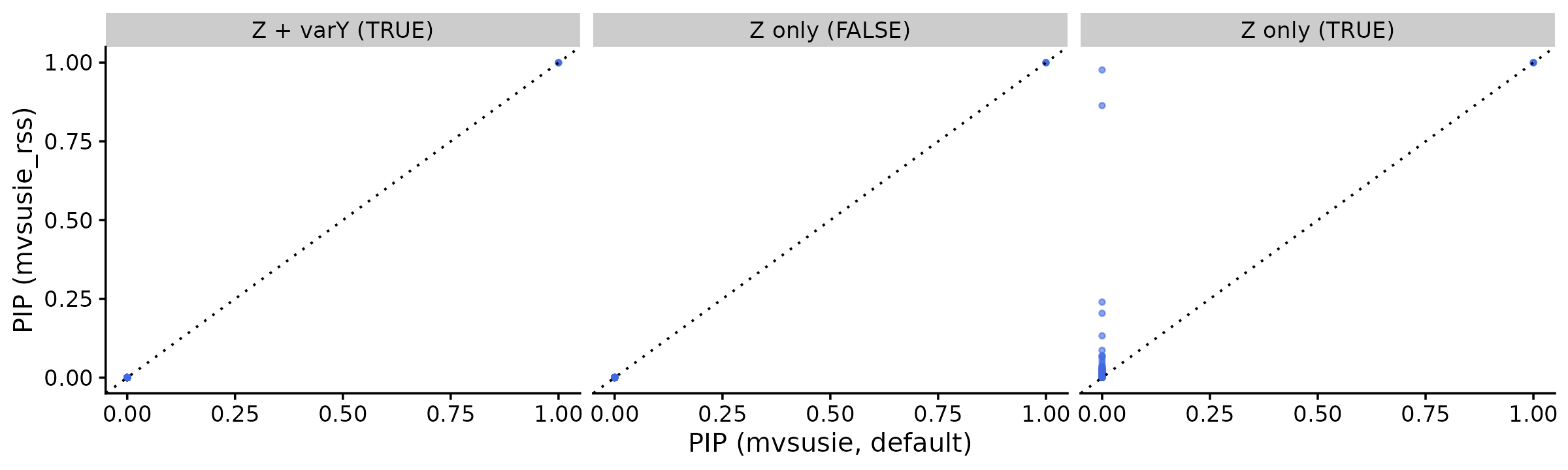
The inflated PIPs from the z-score TRUE path introduce
false discoveries:
check_cs <- function(fit, label) {
  cat(label, ":", length(fit$sets$cs), "credible sets\n")
  for (i in seq_along(fit$sets$cs)) {
    cs <- fit$sets$cs[[i]]
    hit <- intersect(cs, causal)
    status <- if (length(hit) > 0) paste("causal", paste(hit, collapse = ","))
              else "FALSE POSITIVE"
    cat(sprintf("  CS%d: size=%d, purity=%.3f  -> %s\n",
                i, length(cs), fit$sets$purity[i, "min.abs.corr"], status))
  }
  cat("\n")
}
check_cs(fit,       "Individual (TRUE)")
check_cs(fit_rss_f, "Z-only (FALSE)")
check_cs(fit_rss_t, "Z-only (TRUE)")
# Individual (TRUE) : 3 credible sets
#   CS1: size=1, purity=1.000  -> causal 129
#   CS2: size=1, purity=1.000  -> causal 836
#   CS3: size=1, purity=1.000  -> causal 930
#
# Z-only (FALSE) : 3 credible sets
#   CS1: size=1, purity=1.000  -> causal 129
#   CS2: size=1, purity=1.000  -> causal 836
#   CS3: size=1, purity=1.000  -> causal 930
#
# Z-only (TRUE) : 4 credible sets
#   CS1: size=1, purity=1.000  -> causal 129
#   CS2: size=1, purity=1.000  -> causal 836
#   CS3: size=1, purity=1.000  -> causal 930
#   CS4: size=1, purity=1.000  -> FALSE POSITIVE
fp <- which(fit_rss_t$pip > 0.5 & fit$pip < 0.1)
if (length(fp) > 0) {
  cat("Non-causal SNPs with PIP > 0.5 in z-only TRUE path:\n")
  for (s in fp)
    cat(sprintf("  SNP %d: PIP_ind=%.4f, PIP_z(F)=%.4f, PIP_z(T)=%.4f\n",
                s, fit$pip[s], fit_rss_f$pip[s], fit_rss_t$pip[s]))
}
# Non-causal SNPs with PIP > 0.5 in z-only TRUE path:
#   SNP 11: PIP_ind=0.0000, PIP_z(F)=0.0000, PIP_z(T)=0.9769
#   SNP 796: PIP_ind=0.0000, PIP_z(F)=0.0000, PIP_z(T)=0.8637
The individual-level fit and the z-score FALSE path both
identify the same three causal SNPs with no false discoveries. The
z-score TRUE path finds an additional credible set that
does not contain a causal SNP, and assigns high PIPs to
non-causal SNPs.
This illustrates the recommendation from Zou et al.
(2022): when only z-scores and LD are available, fixing the residual
variance (estimate_residual_variance = FALSE) is the safer
default.
Coefficient estimates across interfaces
The Bhat/Shat/varY interface
(3a) produces coefficients on the original scale,
identical to mvsusie(), because the standard errors
Shat carry the genotype scale information needed to
reconstruct the exact sufficient statistics.
The z-score path works on a doubly standardized scale: the z-score Z_{jr} = \hat\beta_{jr}/\mathrm{se}_{jr} absorbs both \mathrm{sd}(X_j) and \mathrm{sd}(Y_r). Internally the path constructs X^TX = (N-1)\,R (correlation matrix) and X^TY = \sqrt{N-1}\,Z, so the fitted coefficients relate to the individual-level ones as
\hat\beta^{\text{ind}}_{jr} \;\approx\; \hat\beta^{Z}_{jr}\;\times\; \frac{\mathrm{sd}(Y_r)}{\mathrm{sd}(X_j)}.
This is not a single constant factor — it varies by both SNP j (through \mathrm{sd}(X_j)) and trait r (through \mathrm{sd}(Y_r)) — so the raw correlation between the vectorized coefficient matrices is less than one even when the PIPs match perfectly.
coef_ind  <- coef(fit)[-1, ]
coef_bhat <- coef(fit_rss_bhat)[-1, ]
coef_z    <- coef(fit_rss_f)[-1, ]

# Rescale z-score coefficients to original scale
csd <- sqrt(colSums(Xc^2) / (n - 1))  # genotype column SDs
sdY <- apply(Y, 2, sd)
coef_z_rescaled <- coef_z
for (j in seq_len(p))
  for (rr in seq_len(r))
    coef_z_rescaled[j, rr] <- coef_z[j, rr] * sdY[rr] / csd[j]

cat("=== Bhat/Shat/varY vs mvsusie (original scale) ===\n")
cat("  max |coef diff|:", max(abs(coef_ind - coef_bhat)), "\n")
cat("  correlation:", round(cor(as.vector(coef_ind),
                                as.vector(coef_bhat)), 6), "\n\n")

cat("=== Z-score vs mvsusie (raw, standardized scale) ===\n")
cat("  correlation:", round(cor(as.vector(coef_ind),
                                as.vector(coef_z)), 4), "\n")
cat("  max |coef| individual:", round(max(abs(coef_ind)), 4), "\n")
cat("  max |coef| z-score:", round(max(abs(coef_z)), 4), "\n\n")

cat("=== Z-score vs mvsusie (after rescaling by sd(Y)/sd(X)) ===\n")
cat("  correlation:", round(cor(as.vector(coef_ind),
                                as.vector(coef_z_rescaled)), 6), "\n")
cat("  max |coef diff|:", round(max(abs(coef_ind - coef_z_rescaled)), 4), "\n")
# === Bhat/Shat/varY vs mvsusie (original scale) ===
#   max |coef diff|: 1.092258e-09
#   correlation: 1
#
# === Z-score vs mvsusie (raw, standardized scale) ===
#   correlation: 0.9596
#   max |coef| individual: 1.1719
#   max |coef| z-score: 0.5545
#
# === Z-score vs mvsusie (after rescaling by sd(Y)/sd(X)) ===
#   correlation: 0.999964
#   max |coef diff|: 0.0168
The Bhat/Shat/varY
coefficients match mvsusie() at machine precision. The raw
z-score coefficients are on a doubly-standardized scale with correlation
\approx 0.96 against
mvsusie(). After rescaling by \mathrm{sd}(Y_r)/\mathrm{sd}(X_j) the
agreement is near-perfect (correlation >
0.9999). The small residual comes from the PVE adjustment applied
to z-scores. In practice this rescaling requires \mathrm{sd}(X) and \mathrm{sd}(Y) which are not available from
summary statistics alone.
pdat <- data.frame(
  coef_ind = rep(as.vector(coef_ind), 3),
  coef_rss = c(as.vector(coef_bhat),
               as.vector(coef_z),
               as.vector(coef_z_rescaled)),
  interface = factor(rep(c("Bhat/Shat/varY\n(original scale)",
                            "Z-score\n(standardized)",
                            "Z-score rescaled\n(sd(Y)/sd(X))"),
                         each = length(coef_ind)),
                     levels = c("Bhat/Shat/varY\n(original scale)",
                                "Z-score\n(standardized)",
                                "Z-score rescaled\n(sd(Y)/sd(X))"))
)
ggplot(pdat, aes(x = coef_ind, y = coef_rss)) +
  geom_point(shape = 20, size = 1.5, color = "royalblue", alpha = 0.6) +
  geom_abline(intercept = 0, slope = 1, linetype = "dotted") +
  facet_wrap(~interface, scales = "free") +
  labs(x = "Coefficient (mvsusie)", y = "Coefficient (mvsusie_rss)") +
  theme_cowplot(font_size = 12)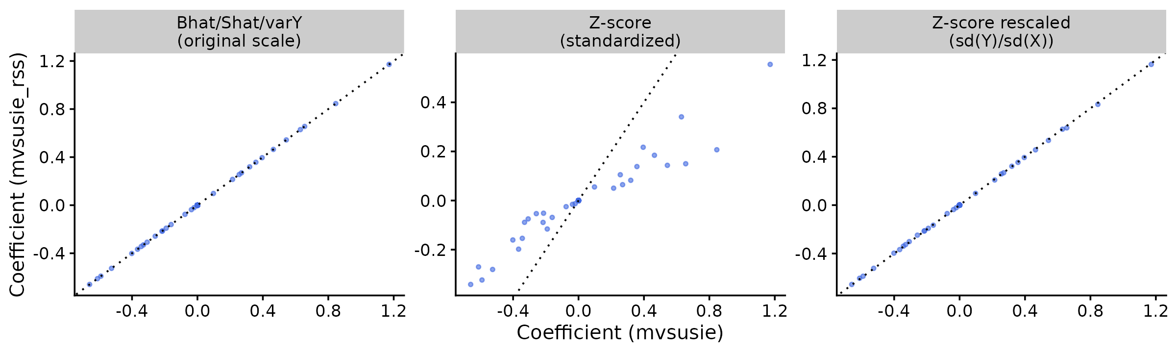
The left panel confirms that
Bhat/Shat/varY recovers the exact
coefficients. The middle panel shows the z-score coefficients are
attenuated due to the doubly-standardized scale. The right panel shows
that rescaling by \mathrm{sd}(Y_r)/\mathrm{sd}(X_j) recovers
the original coefficients almost exactly.
We can also verify this at causal SNPs:
cat("Coefficients at causal SNPs (first 3 traits):\n\n")
for (j in causal) {
  cat(sprintf("SNP %d:\n", j))
  cat("  individual:    ", round(coef_ind[j, 1:3], 4), "\n")
  cat("  Bhat/Shat/varY:", round(coef_bhat[j, 1:3], 4), "\n")
  cat("  z-score raw:   ", round(coef_z[j, 1:3], 4), "\n")
  cat("  z-score rescaled:", round(coef_z_rescaled[j, 1:3], 4), "\n\n")
}
# Coefficients at causal SNPs (first 3 traits):
#
# SNP 129:
#   individual:     0.6293 0.0976 -0.6594
#   Bhat/Shat/varY: 0.6293 0.0976 -0.6594
#   z-score raw:    0.3409 0.0553 -0.3417
#   z-score rescaled: 0.6274 0.097 -0.6556
#
# SNP 679:
#   individual:     0 0 0
#   Bhat/Shat/varY: 0 0 0
#   z-score raw:    0 0 0
#   z-score rescaled: 0 0 0
#
# SNP 836:
#   individual:     0.2554 -0.037 0.3571
#   Bhat/Shat/varY: 0.2554 -0.037 0.3571
#   z-score raw:    0.1051 -0.0156 0.1384
#   z-score rescaled: 0.2577 -0.0365 0.3535
#
# SNP 930:
#   individual:     -0.2138 0.3193 0.6554
#   Bhat/Shat/varY: -0.2138 0.3193 0.6554
#   z-score raw:    -0.0516 0.0824 0.1498
#   z-score rescaled: -0.211 0.3212 0.6385