ELBO, convergence, and model selection

This vignette covers the evidence lower bound (ELBO) used by mvSuSiE for model fitting and convergence monitoring, and compares the EM and optim algorithms for prior variance estimation.

library(mvsusieR)
library(susieR)
library(ggplot2)
library(cowplot)
set.seed(1)

data(simdata)
X <- simdata$raw$X
n <- nrow(X); p <- ncol(X); r <- 10

causal <- sort(sample(p, 3))
B <- matrix(0, p, r)
for (j in causal) B[j, ] <- rnorm(r, 0, 0.5)
Y <- X %*% B + matrix(rnorm(n * r), n, r)

ELBO and convergence

mvSuSiE uses the Iterative Bayesian Stepwise Selection (IBSS) algorithm to maximize the evidence lower bound (ELBO). The ELBO is a lower bound on the log marginal likelihood and should increase monotonically at each iteration.

prior <- create_mixture_prior(R = r)
fit <- mvsusie(X, Y, L = 10,
               prior_variance = prior,
               tol = 1e-4,
               verbose = FALSE)

elbo <- fit$elbo
cat("Iterations:", length(elbo), "\n")
cat("Final ELBO:", tail(elbo, 1), "\n")

pdat <- data.frame(iter = seq_along(elbo), elbo = elbo)
ggplot(pdat, aes(x = iter, y = elbo)) +
  geom_line(color = "royalblue") +
  geom_point(color = "royalblue", size = 2) +
  labs(x = "Iteration", y = "ELBO") +
  theme_cowplot(font_size = 12)

# Iterations: 4 
# Final ELBO: -8294.175

Effect pruning via log Bayes factors

mvSuSiE fits a model with L single effects. Effects that do not contribute to the model have small or negative log Bayes factors (LBF) and are automatically pruned when estimate_prior_variance = TRUE. This makes the model robust to over-specification of L.

cat("L =", length(fit$lbf), "single effects\n")
cat("Log Bayes factors:\n")
for (l in seq_along(fit$lbf)) {
  pruned <- if (fit$V[l] < 1e-9) " [pruned]" else ""
  cat(sprintf("  Effect %d: lbf = %8.2f, V = %.4e%s\n",
              l, fit$lbf[l], fit$V[l], pruned))
}
# L = 10 single effects
# Log Bayes factors:
#   Effect 1: lbf =   178.51, V = 5.8701e-02
#   Effect 2: lbf =   105.96, V = 3.6540e-02
#   Effect 3: lbf =    49.91, V = 2.0270e-02
#   Effect 4: lbf =     0.00, V = 0.0000e+00 [pruned]
#   Effect 5: lbf =     0.00, V = 0.0000e+00 [pruned]
#   Effect 6: lbf =     0.00, V = 0.0000e+00 [pruned]
#   Effect 7: lbf =     0.00, V = 0.0000e+00 [pruned]
#   Effect 8: lbf =     0.00, V = 0.0000e+00 [pruned]
#   Effect 9: lbf =     0.00, V = 0.0000e+00 [pruned]
#   Effect 10: lbf =     0.00, V = 0.0000e+00 [pruned]

lbf_dat <- data.frame(effect = seq_along(fit$lbf),
                       lbf = fit$lbf,
                       active = fit$V > 1e-9)
ggplot(lbf_dat, aes(x = effect, y = lbf, fill = active)) +
  geom_col() +
  scale_fill_manual(values = c("gray70", "royalblue"),
                    labels = c("Pruned", "Active")) +
  labs(x = "Single effect", y = "Log Bayes factor", fill = "") +
  theme_cowplot(font_size = 12)

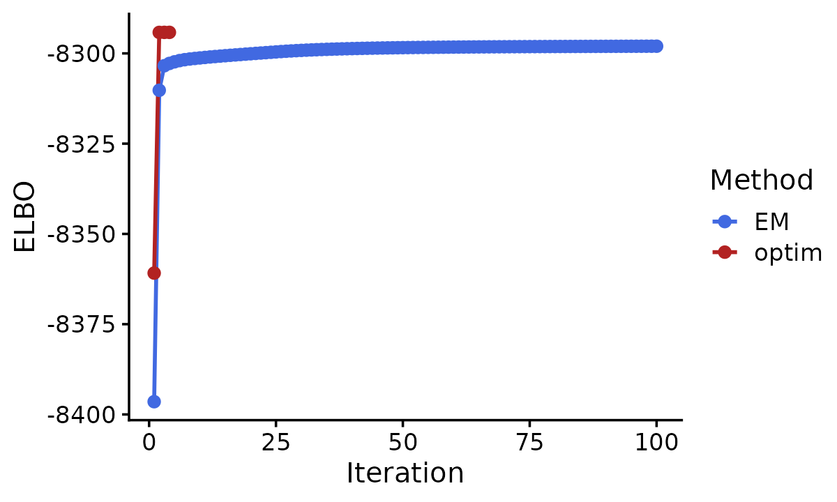
EM vs optim for prior variance estimation

The estimate_prior_variance option (default TRUE) allows mvSuSiE to estimate a scalar multiplier for the prior. mvSuSiE provides two algorithms for estimating the prior variance scaling factor: "EM" (expectation-maximization) and "optim" (Brent optimizer). The optim method typically converges in fewer iterations because it directly maximizes the ELBO with respect to the prior scaling factor at each iteration.

fit_em <- mvsusie(X, Y, L = 10,
                  prior_variance = prior,
                  estimate_prior_method = "EM",
                  tol = 1e-4, verbose = FALSE)
# WARNING: IBSS algorithm did not converge in 100 iterations!
# Warning: IBSS algorithm did not converge in 100 iterations!

fit_optim <- mvsusie(X, Y, L = 10,
                     prior_variance = prior,
                     estimate_prior_method = "optim",
                     tol = 1e-4, verbose = FALSE)

cat("EM: ", length(fit_em$elbo), "iterations, final ELBO =",
    tail(fit_em$elbo, 1), "\n")
cat("optim:", length(fit_optim$elbo), "iterations, final ELBO =",
    tail(fit_optim$elbo, 1), "\n")
# EM:  100 iterations, final ELBO = -8298.009 
# optim: 4 iterations, final ELBO = -8294.175

max_iter <- max(length(fit_em$elbo), length(fit_optim$elbo))
pdat <- data.frame(
  iter = c(seq_along(fit_em$elbo), seq_along(fit_optim$elbo)),
  elbo = c(fit_em$elbo, fit_optim$elbo),
  method = c(rep("EM", length(fit_em$elbo)),
             rep("optim", length(fit_optim$elbo)))
)
ggplot(pdat, aes(x = iter, y = elbo, color = method)) +
  geom_line(linewidth = 0.8) +
  geom_point(size = 2) +
  scale_color_manual(values = c("EM" = "royalblue", "optim" = "firebrick")) +
  labs(x = "Iteration", y = "ELBO", color = "Method") +
  theme_cowplot(font_size = 12)

Gao Wang

2026-05-17

ELBO and convergence

Effect pruning via log Bayes factors

EM vs optim for prior variance estimation