Fine-mapping with SuSiE-ash and SuSiE-inf
Alex McCreight
2026-07-16
Source:vignettes/susie_unmappable_effects.Rmd
susie_unmappable_effects.RmdThis vignette demonstrates how to use the SuSiE-ash and SuSiE-inf models. We use a simulated data set with n = 1000 individuals, p = 5000 variants, and a complex genetic architecture combining 3 sparse, 5 oligogenic, and 15 polygenic effects.
Data
library(susieR)
data(unmappable_data)

X <- unmappable_data$X
y <- as.vector(unmappable_data$y)
b <- unmappable_data$beta

plot(abs(b), ylab = "Absolute Effect Size", pch = 16)
points(which(b != 0), abs(b[b != 0]), col = 2, pch = 16)
Summary Statistics and Z-Scores
Before fitting the models, we can examine the marginal association
statistics. We use univariate_regression() to compute
effect sizes and standard errors, then derive z-scores:
sumstats <- univariate_regression(X, y)
z_scores <- sumstats$betahat / sumstats$sebetahat
The z-scores show the strength of marginal association for each variant. Red points indicate non-zero effect sizes:
susie_plot(z_scores, y = "z", b = b, add_legend = TRUE)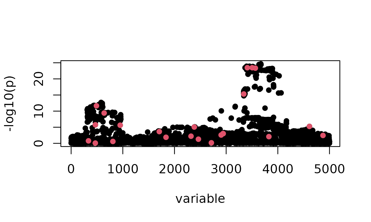
Here we can see the signal landscape before fine-mapping. Note that some causal variants have strong z-scores while others may be weaker or masked by LD with nearby variants.
Notably, variant 2714 has the largest true effect size in the simulation:
strongest_idx <- which.max(abs(b))
cat("Strongest effect variant:", strongest_idx, "\n")
# Strongest effect variant: 2714
cat("True effect size:", round(b[strongest_idx], 3), "\n")
# True effect size: -0.271
cat("Marginal z-score:", round(z_scores[strongest_idx], 3), "\n")
# Marginal z-score: -0.412
cat("Marginal p-value:", format.pval(2 * pnorm(-abs(z_scores[strongest_idx]))), "\n")
# Marginal p-value: 0.68011
Despite having the largest true effect, this variant has a very small marginal z-score and a large p-value. This illustrates a fundamental challenge in fine-mapping: the marginal association of a large-effect causal variant can be masked by other variants in LD, while smaller-effect variants may show stronger marginal signals. This masking makes it difficult to identify the true causal variants from marginal statistics alone.
Step 1: Standard SuSiE and False Positives
We first fit standard SuSiE:
t0 <- proc.time()
fit_susie <- susie(X, y, L = 10)
t1 <- proc.time()
t1 - t0
#    user  system elapsed
#  43.683   0.157  12.632
susie_plot(fit_susie, y = "PIP", b = b, main = "SuSiE (standard)", add_legend = TRUE)
We set L = 10 to allow SuSiE to capture up to 10 sparse
effects. However, given the complex architecture with 23 true causal
variants, this may be insufficient.
To see which true effects the credible sets capture, we plot the CS on the true effect sizes:
plot_cs_effects <- function(fit, b, main = "") {
  colors <- c("dodgerblue2", "green4", "#6A3D9A", "#FF7F00", "gold1", "firebrick2")
  plot(abs(b), pch = 16, ylab = "Absolute Effect Size", main = main)
  if (!is.null(fit$sets$cs)) {
    for (i in rev(seq_along(fit$sets$cs))) {
      cs_idx <- fit$sets$cs[[i]]
      points(cs_idx, abs(b[cs_idx]), col = colors[(i-1) %% 6 + 1], pch = 16, cex = 1.5)
    }
  }

  cat(sprintf("True causals: %s\n", paste(which(b != 0), collapse=", ")))
  for (i in seq_along(fit$sets$cs)) {
    cs_idx <- fit$sets$cs[[i]]
    sentinel <- cs_idx[which.max(fit$pip[cs_idx])]
    tp <- any(b[cs_idx] != 0)
    cat(sprintf("  CS%d: %d %s\n", i, sentinel, ifelse(tp, "TP", "FP")))
  }
}

plot_cs_effects(fit_susie, b, main = "SuSiE CS on true effects")
# True causals: 336, 468, 469, 490, 639, 808, 949, 1706, 1836, 2320, 2383, 2463, 2714, 2903, 2939, 2943, 3341, 3410, 3504, 3565, 3827, 4612, 4874
#   CS1: 3520 TP
#   CS2: 2716 FP
#   CS3: 2386 FP
#   CS4: 960 FP
#   CS5: 447 FP
SuSiE identifies 5 credible sets, but examining them more closely reveals a problem. Many of these credible sets appear to be false positives arising from synthetic associations.
A synthetic association occurs when a non-causal variant shows an association with the phenotype because it is in LD with true causal variants. The non-causal variant “borrows” signal from correlated effect variants, and when it is correlated with multiple effect variants, these contributions can accumulate to create an inflated signal.
Let’s examine one of the false positive credible sets to see this in action:
nonzero_idx <- which(b != 0)
fp_cs <- fit_susie$sets$cs[["L4"]]
top_var <- fp_cs[which.max(fit_susie$pip[fp_cs])]

cat("False positive CS top variant:", top_var, "\n")
# False positive CS top variant: 2716
cat("True effect (beta):", b[top_var], "\n")
# True effect (beta): 0
cat("Z-score:", round(z_scores[top_var], 2), "\n\n")
# Z-score: 3.89

cat("LD with true effect variants and their contributions:\n")
# LD with true effect variants and their contributions:
contributions <- data.frame(
  variant = nonzero_idx,
  r = round(sapply(nonzero_idx, function(v) cor(X[, top_var], X[, v])), 2),
  beta = round(b[nonzero_idx], 2)
)
contributions$r_times_beta <- round(contributions$r * contributions$beta, 2)
contributions <- contributions[order(-abs(contributions$r_times_beta)), ]
print(head(contributions[abs(contributions$r) > 0.1, ], 6), row.names = FALSE)
#  variant     r  beta r_times_beta
#     2714 -0.15 -0.27         0.04
#     2903  0.80  0.04         0.03
#     2939 -0.16 -0.17         0.03
#     3565  0.19 -0.18        -0.03
#     2943 -0.16 -0.10         0.02
#     3410  0.20 -0.08        -0.02
Variant 2716 has no true effect (beta = 0), yet it has a z-score of 3.89. This synthetic signal arises because it is correlated with multiple effect variants. Notice that:
- It has negative LD with negative-effect variants (2714, 2939, 2943), giving positive contributions
- It has positive LD with a positive-effect variant (2903), also giving a positive contribution
These contributions accumulate to create a synthetic signal at the non-causal variant, which SuSiE then incorrectly identifies as a distinct effect. The other false positive credible sets arise from the same artifact.
Step 2: Increasing Purity to Reduce False Positives
One approach to reduce false positives is to increase the purity
threshold. By default, SuSiE uses min_abs_corr = 0.5. Let’s
try min_abs_corr = 0.8:
cs_pure <- susie_get_cs(fit_susie, X = X, min_abs_corr = 0.8)
cat("Number of CSs with purity >= 0.8:", length(cs_pure$cs), "\n")
# Number of CSs with purity >= 0.8: 3
Raising the purity threshold removes some false positives, but not all of them. Some false positive credible sets have high purity because the non-causal variants within them are highly correlated with each other. These sets pass the purity filter yet still fail to contain any true causal variants.
Step 3: Fitting SuSiE-inf
SuSiE-inf models an infinitesimal component to account for unmappable effects:
t0 <- proc.time()
fit_inf <- susie(X, y, L = 10, unmappable_effects = "inf")
# HINT: Switching to PIP-based convergence: unmappable effects models (inf/ash) do not have a well-defined ELBO.
t1 <- proc.time()
t1 - t0
#    user  system elapsed
#  44.339   0.430  11.888
susie_plot(fit_inf, y = "PIP", b = b, main = "SuSiE-inf", add_legend = TRUE)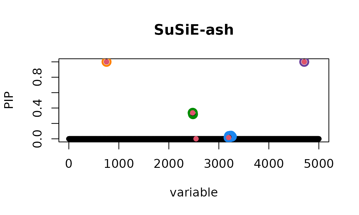
(Note that it may take several minutes to fit the SuSiE-Inf model.)
plot_cs_effects(fit_inf, b, main = "SuSiE-inf CS on true effects")
# True causals: 336, 468, 469, 490, 639, 808, 949, 1706, 1836, 2320, 2383, 2463, 2714, 2903, 2939, 2943, 3341, 3410, 3504, 3565, 3827, 4612, 4874
#   CS1: 2714 TP
SuSiE-inf is more conservative and finds only 1 credible set, eliminating the false positives. However, it also loses the true signal around position 3500 that standard SuSiE correctly identified.
Remarkably, SuSiE-inf identifies the variant with the strongest true effect, the same variant we noted earlier has a very small marginal z-score and large p-value:
if (length(fit_inf$sets$cs) > 0) {
  inf_cs <- fit_inf$sets$cs[[1]]
  cat("SuSiE-inf CS contains variant", strongest_idx, ":", strongest_idx %in% inf_cs, "\n")
  cat("This variant has the largest true effect (beta =", round(b[strongest_idx], 3),
      ") but marginal z-score of only", round(z_scores[strongest_idx], 3), "\n")
}
# SuSiE-inf CS contains variant 2714 : TRUE
# This variant has the largest true effect (beta = -0.271 ) but marginal z-score of only -0.412
This is a striking, as SuSiE-inf recovers the strongest causal signal that is completely invisible in marginal statistics. The intuition is that by modeling background polygenic effects, SuSiE-inf effectively conditions on other variants, revealing signals that are otherwise masked.
However, for other signals, even if we lower the coverage threshold, we cannot recover them, potentially because SuSiE-inf was too aggressive removing them early-on in the SuSiE fit:
for (cov in c(0.9, 0.8, 0.7, 0.5)) {
  cs <- susie_get_cs(fit_inf, X = X, coverage = cov)
  cat(sprintf("Coverage=%.1f: %d credible sets\n", cov, length(cs$cs)))
}
# Coverage=0.9: 1 credible sets
# Coverage=0.8: 1 credible sets
# Coverage=0.7: 1 credible sets
# Coverage=0.5: 1 credible sets
Step 4: SuSiE-ash Achieves the Middle Ground
SuSiE-ash uses adaptive shrinkage to model the unmappable effects, providing a middle ground between standard SuSiE and SuSiE-inf:
t0 <- proc.time()
fit_ash <- susie(X, y, L = 10, unmappable_effects = "ash", verbose = TRUE)
# HINT: For SuSiE-ash, slot_prior was not specified; using default Beta(a=1, b=2), roughly expecting ~3 of 10 slots to be active. Set slot_prior = slot_prior_betabinom(a, b) to override; for an uninformative prior use slot_prior_betabinom(1, 1).
# HINT: Switching to PIP-based convergence: unmappable effects models (inf/ash) do not have a well-defined ELBO.
# iter          ELBO       delta   sigma2      mem      V
#    1     -982.5674           -   0.4674      0.23 GB  [4.36e-02, 1.75e-02, 1.16e-02, 4.12e-03, 2.08e-03, 1.54e-03, 1.22e-03, 9.88e-04, 8.14e-04, 6.76e-04], c_hat=[1.00,1.00,1.00,0.77,0.66,0.64,0.64,0.65,0.67,0.69], lbf=[41.0,12.2,6.3,1.2,0.5,0.3,0.2,0.2,0.1,0.1], C_hat=7.7(10>0.5)
# Mr.ASH terminated at iteration 20: max|beta|=4.0150e-03, sigma2=3.6691e-01, pi0=0.9811
# iter   2: max|d(alpha,PIP)|=2.85e-01, V=[4.52e-02, 1.56e-02, 1.25e-02, 9.49e-03, 0 x 6], c_hat=[1.00,1.00,1.00,0.99,0.69,0.69,0.70,0.70,0.71,0.71], lbf=[55.8,14.1,10.6,4.6,0.0,0.0,0.0,0.0,0.0,0.0], C_hat=8.2(10>0.5) [mem: 0.23 GB]
# Mr.ASH terminated at iteration 15: max|beta|=3.2743e-03, sigma2=3.7299e-01, pi0=0.9876
# iter   3: max|d(alpha,PIP)|=3.15e-01, V=[5.01e-02, 1.68e-02, 1.30e-02, 1.32e-02, 0 x 6], c_hat=[1.00,1.00,1.00,1.00,0.71,0.71,0.71,0.71,0.71,0.71], lbf=[61.4,15.4,11.0,8.8,0.0,0.0,0.0,0.0,0.0,0.0], C_hat=8.3(10>0.5) [mem: 0.24 GB]
# Mr.ASH terminated at iteration 14: max|beta|=3.1254e-03, sigma2=3.7324e-01, pi0=0.9879
# iter   4: max|d(alpha,PIP)|=2.97e-01, V=[5.39e-02, 1.68e-02, 1.33e-02, 1.14e-02, 0 x 6], c_hat=[1.00,1.00,1.00,1.00,0.71,0.71,0.71,0.71,0.71,0.71], lbf=[66.3,15.3,11.4,6.6,0.0,0.0,0.0,0.0,0.0,0.0], C_hat=8.3(10>0.5) [mem: 0.24 GB]
# Mr.ASH terminated at iteration 13: max|beta|=3.1064e-03, sigma2=3.7326e-01, pi0=0.9879
# iter   5: max|d(alpha,PIP)|=2.96e-01, V=[5.40e-02, 1.70e-02, 1.21e-02, 1.12e-02, 0 x 6], c_hat=[1.00,1.00,1.00,1.00,0.71,0.71,0.71,0.71,0.71,0.71], lbf=[66.4,15.7,10.0,6.3,0.0,0.0,0.0,0.0,0.0,0.0], C_hat=8.3(10>0.5) [mem: 0.24 GB]
# Mr.ASH terminated at iteration 13: max|beta|=3.0983e-03, sigma2=3.7322e-01, pi0=0.9879
# iter   6: max|d(alpha,PIP)|=2.96e-01, V=[5.38e-02, 1.69e-02, 1.21e-02, 1.12e-02, 0 x 6], c_hat=[1.00,1.00,1.00,1.00,0.71,0.71,0.71,0.71,0.71,0.71], lbf=[66.2,15.5,9.9,6.3,0.0,0.0,0.0,0.0,0.0,0.0], C_hat=8.3(10>0.5) [mem: 0.24 GB]
# Mr.ASH terminated at iteration 13: max|beta|=3.1041e-03, sigma2=3.7325e-01, pi0=0.9879
# iter   7: max|d(alpha,PIP)|=2.91e-01, V=[5.75e-02, 1.64e-02, 1.23e-02, 1.68e-03, 0 x 6], c_hat=[1.00,1.00,1.00,0.73,0.69,0.69,0.69,0.69,0.68,0.68], lbf=[71.1,14.9,10.3,0.2,0.0,0.0,0.0,0.0,0.0,0.0], C_hat=7.8(10>0.5) [mem: 0.24 GB]
# Mr.ASH terminated at iteration 13: max|beta|=3.0911e-03, sigma2=3.7327e-01, pi0=0.9878
# iter   8: max|d(alpha,PIP)|=3.49e-01, V=[4.99e-02, 1.71e-02, 1.28e-02, 6.23e-04, 0 x 6], c_hat=[1.00,1.00,1.00,0.68,0.68,0.67,0.67,0.67,0.67,0.67], lbf=[61.1,15.7,10.8,0.0,0.0,0.0,0.0,0.0,0.0,0.0], C_hat=7.7(10>0.5) [mem: 0.24 GB]
# Mr.ASH terminated at iteration 13: max|beta|=3.1077e-03, sigma2=3.7321e-01, pi0=0.9880
# iter   9: max|d(alpha,PIP)|=3.30e-01, V=[4.74e-02, 1.77e-02, 1.27e-02, 7.09e-04, 0 x 6], c_hat=[1.00,1.00,1.00,0.68,0.67,0.67,0.67,0.67,0.67,0.67], lbf=[57.7,16.4,10.7,0.0,0.0,0.0,0.0,0.0,0.0,0.0], C_hat=7.7(10>0.5) [mem: 0.24 GB]
# Mr.ASH terminated at iteration 13: max|beta|=3.1094e-03, sigma2=3.7324e-01, pi0=0.9881
# iter  10: max|d(alpha,PIP)|=3.27e-01, V=[4.69e-02, 1.79e-02, 1.27e-02, 7.95e-04, 0 x 6], c_hat=[1.00,1.00,1.00,0.68,0.67,0.67,0.67,0.67,0.67,0.67], lbf=[57.0,16.7,10.7,0.0,0.0,0.0,0.0,0.0,0.0,0.0], C_hat=7.7(10>0.5) [mem: 0.24 GB]
# Mr.ASH terminated at iteration 13: max|beta|=3.1115e-03, sigma2=3.7327e-01, pi0=0.9881
# iter  11: max|d(alpha,PIP)|=3.27e-01, V=[4.68e-02, 1.80e-02, 1.27e-02, 8.19e-04, 0 x 6], c_hat=[1.00,1.00,1.00,0.68,0.67,0.67,0.67,0.67,0.67,0.67], lbf=[57.0,16.8,10.7,0.0,0.0,0.0,0.0,0.0,0.0,0.0], C_hat=7.7(10>0.5) [mem: 0.24 GB]
# Mr.ASH terminated at iteration 13: max|beta|=3.1122e-03, sigma2=3.7328e-01, pi0=0.9881
# iter  12: max|d(alpha,PIP)|=8.72e-02, V=[4.68e-02, 1.80e-02, 1.27e-02, 8.22e-04, 0 x 6], c_hat=[1.00,1.00,1.00,0.68,0.67,0.67,0.67,0.67,0.67,0.67], lbf=[56.9,16.8,10.7,0.0,0.0,0.0,0.0,0.0,0.0,0.0], C_hat=7.7(10>0.5) [mem: 0.24 GB]
# Mr.ASH terminated at iteration 13: max|beta|=3.1122e-03, sigma2=3.7328e-01, pi0=0.9881
# iter  13: max|d(alpha,PIP)|=4.45e-05, V=[4.68e-02, 1.80e-02, 1.27e-02, 8.23e-04, 0 x 6], c_hat=[1.00,1.00,1.00,0.68,0.67,0.67,0.67,0.67,0.67,0.67], lbf=[56.9,16.8,10.7,0.0,0.0,0.0,0.0,0.0,0.0,0.0], C_hat=7.7(10>0.5) -- converged (alpha_pip_fixed_point) [mem: 0.24 GB]
# Mr.ASH terminated at iteration 9: max|beta|=2.6093e-03, sigma2=3.6708e-01, pi0=0.9906
t1 <- proc.time()
t1 - t0
#    user  system elapsed
#  95.141   2.897  50.394
susie_plot(fit_ash, y = "PIP", b = b, main = "SuSiE-ash", add_legend = TRUE)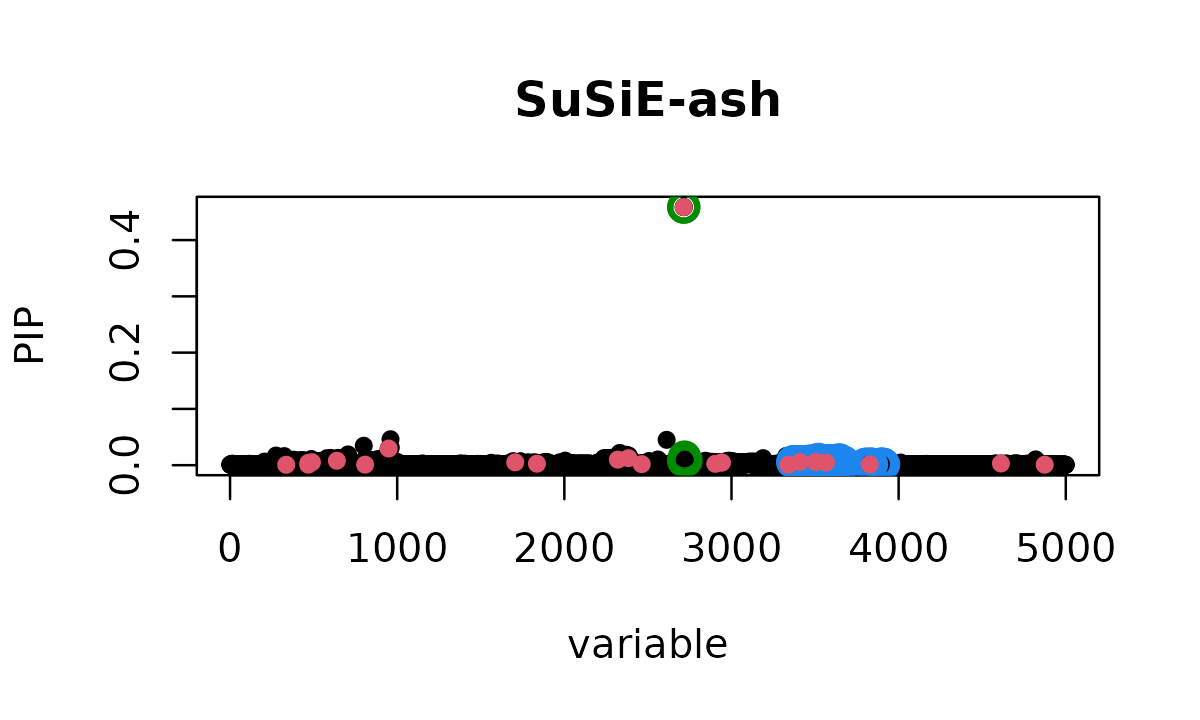
(Note that it may take several minutes to fit the SuSiE-ash model.)
plot_cs_effects(fit_ash, b, main = "SuSiE-ash CS on true effects")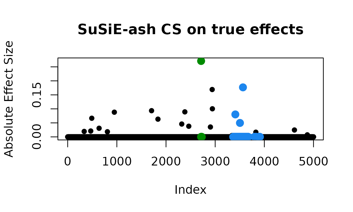
# True causals: 336, 468, 469, 490, 639, 808, 949, 1706, 1836, 2320, 2383, 2463, 2714, 2903, 2939, 2943, 3341, 3410, 3504, 3565, 3827, 4612, 4874
#   CS1: 3671 TP
#   CS2: 603 TP
#   CS3: 2386 TP
SuSiE-ash finds 3 correct credible sets.
Still, it does not discover all 23 causal variants, nor does it recover the strongest effect (variant 2714) that SuSiE-inf found. However, the adaptive shrinkage approach allows SuSiE-ash to distinguish between true sparse signals and the polygenic background more effectively than either standard SuSiE or SuSiE-inf alone.
SuSiE-ash can also be used with summary statistics via
susie_ss(), using mr.ash.rss as the backend
for the adaptive shrinkage component. This enables fine-mapping with
unmappable effects when only sufficient statistics (X’X, X’y, y’y) are
available.
XtX <- crossprod(X)
Xty <- crossprod(X, y)
yty <- sum(y^2)
n <- nrow(X)

t0 <- proc.time()
fit_ash_ss <- susie_ss(XtX = XtX, Xty = Xty, yty = yty, n = n,
                        L = 10, unmappable_effects = "ash", verbose = TRUE)
# HINT: For SuSiE-ash, slot_prior was not specified; using default Beta(a=1, b=2), roughly expecting ~3 of 10 slots to be active. Set slot_prior = slot_prior_betabinom(a, b) to override; for an uninformative prior use slot_prior_betabinom(1, 1).
# HINT: Switching to PIP-based convergence: unmappable effects models (inf/ash) do not have a well-defined ELBO.
# iter          ELBO       delta   sigma2      mem      V
#    1     -982.7939           -   0.4676      0.57 GB  [4.36e-02, 1.75e-02, 1.16e-02, 4.12e-03, 2.08e-03, 1.54e-03, 1.22e-03, 9.88e-04, 8.14e-04, 6.76e-04], c_hat=[1.00,1.00,1.00,0.77,0.66,0.64,0.64,0.65,0.67,0.69], lbf=[40.9,12.2,6.3,1.2,0.5,0.3,0.2,0.2,0.1,0.1], C_hat=7.7(10>0.5)
# iter   2: max|d(alpha,PIP)|=2.84e-01, V=[4.51e-02, 1.56e-02, 1.25e-02, 9.46e-03, 0 x 6], c_hat=[1.00,1.00,1.00,0.99,0.69,0.69,0.70,0.70,0.71,0.71], lbf=[55.8,14.1,10.6,4.5,0.0,0.0,0.0,0.0,0.0,0.0], C_hat=8.2(10>0.5) [mem: 0.57 GB]
# iter   3: max|d(alpha,PIP)|=3.15e-01, V=[5.01e-02, 1.68e-02, 1.30e-02, 1.32e-02, 0 x 6], c_hat=[1.00,1.00,1.00,1.00,0.71,0.71,0.71,0.71,0.71,0.71], lbf=[61.3,15.4,11.0,8.8,0.0,0.0,0.0,0.0,0.0,0.0], C_hat=8.3(10>0.5) [mem: 0.57 GB]
# iter   4: max|d(alpha,PIP)|=2.97e-01, V=[5.38e-02, 1.68e-02, 1.33e-02, 1.14e-02, 0 x 6], c_hat=[1.00,1.00,1.00,1.00,0.71,0.71,0.71,0.71,0.71,0.71], lbf=[66.2,15.3,11.4,6.5,0.0,0.0,0.0,0.0,0.0,0.0], C_hat=8.3(10>0.5) [mem: 0.57 GB]
# iter   5: max|d(alpha,PIP)|=2.96e-01, V=[5.40e-02, 1.70e-02, 1.21e-02, 1.12e-02, 0 x 6], c_hat=[1.00,1.00,1.00,1.00,0.71,0.71,0.71,0.71,0.71,0.71], lbf=[66.4,15.7,10.0,6.3,0.0,0.0,0.0,0.0,0.0,0.0], C_hat=8.3(10>0.5) [mem: 0.57 GB]
# iter   6: max|d(alpha,PIP)|=2.96e-01, V=[5.38e-02, 1.69e-02, 1.20e-02, 1.12e-02, 0 x 6], c_hat=[1.00,1.00,1.00,1.00,0.71,0.71,0.71,0.71,0.71,0.71], lbf=[66.1,15.5,9.9,6.3,0.0,0.0,0.0,0.0,0.0,0.0], C_hat=8.3(10>0.5) [mem: 0.57 GB]
# iter   7: max|d(alpha,PIP)|=2.90e-01, V=[5.75e-02, 1.64e-02, 1.23e-02, 1.68e-03, 0 x 6], c_hat=[1.00,1.00,1.00,0.73,0.69,0.69,0.69,0.69,0.68,0.68], lbf=[71.0,14.9,10.3,0.2,0.0,0.0,0.0,0.0,0.0,0.0], C_hat=7.8(10>0.5) [mem: 0.57 GB]
# iter   8: max|d(alpha,PIP)|=3.49e-01, V=[4.99e-02, 1.71e-02, 1.28e-02, 6.23e-04, 0 x 6], c_hat=[1.00,1.00,1.00,0.68,0.68,0.67,0.67,0.67,0.67,0.67], lbf=[61.0,15.7,10.8,0.0,0.0,0.0,0.0,0.0,0.0,0.0], C_hat=7.7(10>0.5) [mem: 0.57 GB]
# iter   9: max|d(alpha,PIP)|=3.30e-01, V=[4.74e-02, 1.77e-02, 1.27e-02, 7.06e-04, 0 x 6], c_hat=[1.00,1.00,1.00,0.68,0.67,0.67,0.67,0.67,0.67,0.67], lbf=[57.7,16.4,10.7,0.0,0.0,0.0,0.0,0.0,0.0,0.0], C_hat=7.7(10>0.5) [mem: 0.57 GB]
# iter  10: max|d(alpha,PIP)|=3.27e-01, V=[4.68e-02, 1.79e-02, 1.27e-02, 7.91e-04, 0 x 6], c_hat=[1.00,1.00,1.00,0.68,0.67,0.67,0.67,0.67,0.67,0.67], lbf=[57.0,16.7,10.7,0.0,0.0,0.0,0.0,0.0,0.0,0.0], C_hat=7.7(10>0.5) [mem: 0.57 GB]
# iter  11: max|d(alpha,PIP)|=3.27e-01, V=[4.68e-02, 1.80e-02, 1.27e-02, 8.15e-04, 0 x 6], c_hat=[1.00,1.00,1.00,0.68,0.67,0.67,0.67,0.67,0.67,0.67], lbf=[56.9,16.8,10.7,0.0,0.0,0.0,0.0,0.0,0.0,0.0], C_hat=7.7(10>0.5) [mem: 0.57 GB]
# iter  12: max|d(alpha,PIP)|=8.71e-02, V=[4.68e-02, 1.80e-02, 1.27e-02, 8.19e-04, 0 x 6], c_hat=[1.00,1.00,1.00,0.68,0.67,0.67,0.67,0.67,0.67,0.67], lbf=[56.9,16.8,10.7,0.0,0.0,0.0,0.0,0.0,0.0,0.0], C_hat=7.7(10>0.5) [mem: 0.57 GB]
# iter  13: max|d(alpha,PIP)|=4.49e-05, V=[4.68e-02, 1.80e-02, 1.27e-02, 8.19e-04, 0 x 6], c_hat=[1.00,1.00,1.00,0.68,0.67,0.67,0.67,0.67,0.67,0.67], lbf=[56.9,16.8,10.7,0.0,0.0,0.0,0.0,0.0,0.0,0.0], C_hat=7.7(10>0.5) -- converged (alpha_pip_fixed_point) [mem: 0.57 GB]
t1 <- proc.time()
t1 - t0
#    user  system elapsed
# 194.813   3.548  74.758
susie_plot(fit_ash_ss, y = "PIP", b = b, main = "SuSiE-ash (SS)", add_legend = TRUE)
plot_cs_effects(fit_ash_ss, b, main = "SuSiE-ash (SS) CS on true effects")
# True causals: 336, 468, 469, 490, 639, 808, 949, 1706, 1836, 2320, 2383, 2463, 2714, 2903, 2939, 2943, 3341, 3410, 3504, 3565, 3827, 4612, 4874
#   CS1: 3671 TP
#   CS2: 603 TP
#   CS3: 2386 TP
We can verify the agreement between the two approaches:
pip_ind <- susie_get_pip(fit_ash)
pip_ss <- susie_get_pip(fit_ash_ss)
cat("Max |PIP difference|:", max(abs(pip_ind - pip_ss)), "\n")
# Max |PIP difference|: 8.393242e-05
cat("PIP correlation:", cor(pip_ind, pip_ss), "\n")
# PIP correlation: 0.9999999
cat("Max |theta difference|:", max(abs(fit_ash$theta - fit_ash_ss$theta)), "\n")
# Max |theta difference|: 3.35643e-06
When only GWAS summary statistics are available,
susie_rss() can be used. For best agreement with
individual-level analysis, we recommend providing effect sizes
(bhat), standard errors (shat), and the
phenotypic variance (var_y) along with the in-sample LD
matrix (R) and sample size (n). This preserves
the original data scale, allowing the adaptive shrinkage component to
calibrate correctly:
R <- cor(X)
bhat <- sumstats$betahat
shat <- sumstats$sebetahat

t0 <- proc.time()
fit_ash_rss <- susie_rss(bhat = bhat, shat = shat, R = R,
                          var_y = var(y), n = n,
                          L = 10, unmappable_effects = "ash",
                          estimate_residual_variance = TRUE, verbose = TRUE)
# HINT: Setting max_iter = 50 for the SuSiE RSS model because slow convergence is often a sign of unstable summary-statistics fitting. To disable this message, explicitly set max_iter = 50 or another value in the susie_rss() call.
# WARNING: estimate_residual_variance = TRUE is not recommended unless R is the "in-sample" R matrix; that is, the correlation matrix obtained using the exact same data matrix X that was used for the other summary statistics. If R is in-sample, set R_finite = FALSE to silence this warning. When covariates are included in the univariate regressions that produced the summary statistics, also consider removing these effects from X before computing R.
# HINT: For SuSiE-ash, slot_prior was not specified; using default Beta(a=1, b=2), roughly expecting ~3 of 10 slots to be active. Set slot_prior = slot_prior_betabinom(a, b) to override; for an uninformative prior use slot_prior_betabinom(1, 1).
# HINT: Switching to PIP-based convergence: unmappable effects models (inf/ash) do not have a well-defined ELBO.
# iter          ELBO       delta   sigma2      mem      V
#    1     -982.5674           -   0.4674      0.76 GB  [4.36e-02, 1.75e-02, 1.16e-02, 4.12e-03, 2.08e-03, 1.54e-03, 1.22e-03, 9.88e-04, 8.14e-04, 6.76e-04], c_hat=[1.00,1.00,1.00,0.77,0.66,0.64,0.64,0.65,0.67,0.69], lbf=[41.0,12.2,6.3,1.2,0.5,0.3,0.2,0.2,0.1,0.1], C_hat=7.7(10>0.5)
# iter   2: max|d(alpha,PIP)|=2.84e-01, V=[4.51e-02, 1.56e-02, 1.25e-02, 9.46e-03, 0 x 6], c_hat=[1.00,1.00,1.00,0.99,0.69,0.69,0.70,0.70,0.71,0.71], lbf=[55.8,14.1,10.6,4.5,0.0,0.0,0.0,0.0,0.0,0.0], C_hat=8.2(10>0.5) [mem: 0.76 GB]
# iter   3: max|d(alpha,PIP)|=3.15e-01, V=[5.01e-02, 1.68e-02, 1.30e-02, 1.32e-02, 0 x 6], c_hat=[1.00,1.00,1.00,1.00,0.71,0.71,0.71,0.71,0.71,0.71], lbf=[61.4,15.4,11.0,8.8,0.0,0.0,0.0,0.0,0.0,0.0], C_hat=8.3(10>0.5) [mem: 0.76 GB]
# iter   4: max|d(alpha,PIP)|=2.97e-01, V=[5.38e-02, 1.68e-02, 1.33e-02, 1.14e-02, 0 x 6], c_hat=[1.00,1.00,1.00,1.00,0.71,0.71,0.71,0.71,0.71,0.71], lbf=[66.3,15.3,11.4,6.6,0.0,0.0,0.0,0.0,0.0,0.0], C_hat=8.3(10>0.5) [mem: 0.76 GB]
# iter   5: max|d(alpha,PIP)|=2.96e-01, V=[5.40e-02, 1.70e-02, 1.21e-02, 1.12e-02, 0 x 6], c_hat=[1.00,1.00,1.00,1.00,0.71,0.71,0.71,0.71,0.71,0.71], lbf=[66.4,15.7,10.0,6.3,0.0,0.0,0.0,0.0,0.0,0.0], C_hat=8.3(10>0.5) [mem: 0.76 GB]
# iter   6: max|d(alpha,PIP)|=2.96e-01, V=[5.38e-02, 1.69e-02, 1.20e-02, 1.12e-02, 0 x 6], c_hat=[1.00,1.00,1.00,1.00,0.71,0.71,0.71,0.71,0.71,0.71], lbf=[66.2,15.5,9.9,6.3,0.0,0.0,0.0,0.0,0.0,0.0], C_hat=8.3(10>0.5) [mem: 0.76 GB]
# iter   7: max|d(alpha,PIP)|=2.90e-01, V=[5.75e-02, 1.64e-02, 1.23e-02, 1.68e-03, 0 x 6], c_hat=[1.00,1.00,1.00,0.73,0.69,0.69,0.69,0.69,0.68,0.68], lbf=[71.1,14.9,10.3,0.2,0.0,0.0,0.0,0.0,0.0,0.0], C_hat=7.8(10>0.5) [mem: 0.76 GB]
# iter   8: max|d(alpha,PIP)|=3.49e-01, V=[4.99e-02, 1.71e-02, 1.28e-02, 6.24e-04, 0 x 6], c_hat=[1.00,1.00,1.00,0.68,0.68,0.67,0.67,0.67,0.67,0.67], lbf=[61.1,15.7,10.8,0.0,0.0,0.0,0.0,0.0,0.0,0.0], C_hat=7.7(10>0.5) [mem: 0.76 GB]
# iter   9: max|d(alpha,PIP)|=3.30e-01, V=[4.74e-02, 1.77e-02, 1.27e-02, 7.06e-04, 0 x 6], c_hat=[1.00,1.00,1.00,0.68,0.67,0.67,0.67,0.67,0.67,0.67], lbf=[57.7,16.4,10.7,0.0,0.0,0.0,0.0,0.0,0.0,0.0], C_hat=7.7(10>0.5) [mem: 0.76 GB]
# iter  10: max|d(alpha,PIP)|=3.27e-01, V=[4.69e-02, 1.79e-02, 1.27e-02, 7.92e-04, 0 x 6], c_hat=[1.00,1.00,1.00,0.68,0.67,0.67,0.67,0.67,0.67,0.67], lbf=[57.0,16.7,10.7,0.0,0.0,0.0,0.0,0.0,0.0,0.0], C_hat=7.7(10>0.5) [mem: 0.76 GB]
# iter  11: max|d(alpha,PIP)|=3.27e-01, V=[4.68e-02, 1.80e-02, 1.27e-02, 8.15e-04, 0 x 6], c_hat=[1.00,1.00,1.00,0.68,0.67,0.67,0.67,0.67,0.67,0.67], lbf=[57.0,16.8,10.7,0.0,0.0,0.0,0.0,0.0,0.0,0.0], C_hat=7.7(10>0.5) [mem: 0.76 GB]
# iter  12: max|d(alpha,PIP)|=8.72e-02, V=[4.68e-02, 1.80e-02, 1.27e-02, 8.19e-04, 0 x 6], c_hat=[1.00,1.00,1.00,0.68,0.67,0.67,0.67,0.67,0.67,0.67], lbf=[56.9,16.8,10.7,0.0,0.0,0.0,0.0,0.0,0.0,0.0], C_hat=7.7(10>0.5) [mem: 0.76 GB]
# iter  13: max|d(alpha,PIP)|=4.50e-05, V=[4.68e-02, 1.80e-02, 1.27e-02, 8.19e-04, 0 x 6], c_hat=[1.00,1.00,1.00,0.68,0.67,0.67,0.67,0.67,0.67,0.67], lbf=[56.9,16.8,10.7,0.0,0.0,0.0,0.0,0.0,0.0,0.0], C_hat=7.7(10>0.5) -- converged (alpha_pip_fixed_point) [mem: 0.76 GB]
t1 <- proc.time()
t1 - t0
#    user  system elapsed
# 193.291   3.804  73.052
susie_plot(fit_ash_rss, y = "PIP", b = b, main = "SuSiE-ash (RSS)", add_legend = TRUE)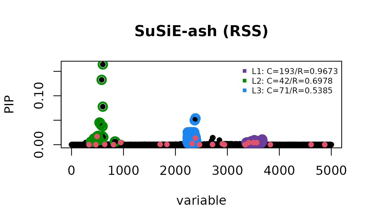
plot_cs_effects(fit_ash_rss, b, main = "SuSiE-ash (RSS) CS on true effects")
# True causals: 336, 468, 469, 490, 639, 808, 949, 1706, 1836, 2320, 2383, 2463, 2714, 2903, 2939, 2943, 3341, 3410, 3504, 3565, 3827, 4612, 4874
#   CS1: 3671 TP
#   CS2: 603 TP
#   CS3: 2386 TP
With bhat, shat, var_y, and
in-sample LD, susie_rss results match susie_ss
closely:
pip_rss <- susie_get_pip(fit_ash_rss)
cat("Max |PIP difference| (SS vs RSS):", max(abs(pip_ss - pip_rss)), "\n")
# Max |PIP difference| (SS vs RSS): 0.0001144609
cat("PIP correlation (SS vs RSS):", cor(pip_ss, pip_rss), "\n")
# PIP correlation (SS vs RSS): 0.9999999
When only z-scores and an LD matrix are available (without
bhat, shat, or var_y),
susie_rss operates on a standardized scale where
var(y) = 1. The credible sets are typically still correct,
but the estimated sigma2 will be on the standardized scale
rather than the original scale. Note that when the LD matrix is not
computed from the same sample as the summary statistics (out-of-sample
LD), setting estimate_residual_variance = FALSE may be more
appropriate to avoid bias from LD mismatch.
Summary
| Method | Credible Sets | False Positives |
|---|---|---|
| SuSiE (purity=0.5) | 5 | 4 |
| SuSiE (purity=0.8) | 3 | 2 |
| SuSiE-inf | 1 | 0 |
| SuSiE-ash | 3 | 0 |
| SuSiE-ash (SS) | 3 | 0 |
| SuSiE-ash (RSS) | 3 | 0 |
What if we increase L for standard SuSiE?
Since the true simulation has 23 causal variants, one might ask: what
if we simply increase L to give SuSiE more capacity? Let’s
try L = 40:
t0 <- proc.time()
fit_susie_L40 <- susie(X, y, L = 40)
t1 <- proc.time()
t1 - t0
#    user  system elapsed
# 564.335   1.325 147.537
susie_plot(fit_susie_L40, y = "PIP", b = b, main = "SuSiE (L=40)", add_legend = TRUE)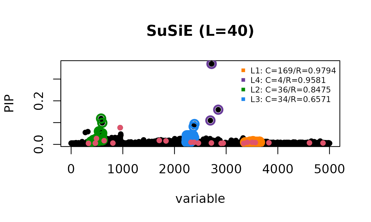
plot_cs_effects(fit_susie_L40, b, main = "SuSiE L=40 CS on true effects")
# True causals: 336, 468, 469, 490, 639, 808, 949, 1706, 1836, 2320, 2383, 2463, 2714, 2903, 2939, 2943, 3341, 3410, 3504, 3565, 3827, 4612, 4874
#   CS1: 3520 TP
#   CS2: 2716 FP
#   CS3: 580 TP
#   CS4: 2386 FP
With L = 40, standard SuSiE does improve! Now it
captures 4 CS with two of them true positives. However, it still
produces false positives and takes considerably longer to converge.
The rationale for SuSiE-ash is to avoid this concern: rather than
specifying a large L to account for all potential effects,
we use a reasonable L for sparse signals and let the
adaptive shrinkage component absorb effects that cannot be mapped due to
insufficiently specified L. This provides a more principled
and computationally efficient approach.
Naturally as a result, SuSiE-ash is more robust to the choice of
L compared to SuSiE. For this example, setting
L anywhere from 5 to 40 yields similar results, unlike
standard SuSiE where performance varies substantially with
L. (Readers can verify this on their own with this
data-set)
Session Information
sessionInfo()
# R version 4.4.3 (2025-02-28)
# Platform: x86_64-conda-linux-gnu
# Running under: Ubuntu 24.04.4 LTS
#
# Matrix products: default
# BLAS/LAPACK: /home/runner/work/susieR/susieR/.pixi/envs/r44/lib/libopenblasp-r0.3.33.so;  LAPACK version 3.12.0
#
# locale:
#  [1] LC_CTYPE=C.UTF-8       LC_NUMERIC=C           LC_TIME=C.UTF-8
#  [4] LC_COLLATE=C.UTF-8     LC_MONETARY=C.UTF-8    LC_MESSAGES=C.UTF-8
#  [7] LC_PAPER=C.UTF-8       LC_NAME=C              LC_ADDRESS=C
# [10] LC_TELEPHONE=C         LC_MEASUREMENT=C.UTF-8 LC_IDENTIFICATION=C
#
# time zone: Etc/UTC
# tzcode source: system (glibc)
#
# attached base packages:
# [1] stats     graphics  grDevices utils     datasets  methods   base
#
# other attached packages:
# [1] susieR_0.16.5
#
# loaded via a namespace (and not attached):
#  [1] Matrix_1.7-5          gtable_0.3.6          jsonlite_2.0.0
#  [4] compiler_4.4.3        crayon_1.5.3          Rcpp_1.1.2
#  [7] jquerylib_0.1.4       systemfonts_1.3.2     scales_1.4.0
# [10] textshaping_1.0.5     yaml_2.3.12           fastmap_1.2.0
# [13] lattice_0.22-9        plyr_1.8.9            ggplot2_4.0.3
# [16] R6_2.6.1              mixsqp_0.3-54         knitr_1.51
# [19] htmlwidgets_1.6.4     desc_1.4.3            zigg_0.0.2
# [22] bslib_0.11.0          RColorBrewer_1.1-3    rlang_1.3.0
# [25] reshape_0.8.10        cachem_1.1.0          xfun_0.60
# [28] fs_2.1.0              sass_0.4.10           S7_0.2.2
# [31] RcppParallel_5.1.11-2 otel_0.2.0            cli_3.6.6
# [34] pkgdown_2.2.1         digest_0.6.39         grid_4.4.3
# [37] irlba_2.3.7           lifecycle_1.0.5       vctrs_0.7.3
# [40] Rfast_2.1.5.2         evaluate_1.0.5        glue_1.8.1
# [43] farver_2.1.2          ragg_1.5.2            rmarkdown_2.31
# [46] matrixStats_1.5.0     tools_4.4.3           htmltools_0.5.9