Accounting for uncertainty in residual variances for small sample studies
William R.P. Denault
2026-07-16
Source:vignettes/small_sample.Rmd
small_sample.RmdThis is vignette is a modified example based on Figure 1 panel B-C-D in Denault et al paper.
For reproducibility, set the seed:
set.seed(1)Data
In this example, we analyze a simulated eQTL data set. The goal is to finemap causal variants for expression (eQTLs).
Baseline SuSiE fit
The original SuSiE method displays signs of misscalibration: the result is highly suspicious as we find 10 credible sets in a data set containing only 47 samples.
res_susie <- susie(X,y,L = 10,verbose = TRUE)
res_susie$sets$cs
# $L2
# [1] 6902
#
# $L3
# [1] 3258
#
# $L5
# [1] 4703
#
# $L7
# [1] 3288
#
# $L9
# [1] 2361
#
# $L1
# [1] 4919 4920
#
# $L6
# [1] 5174 5181 5184
#
# $L8
#  [1] 3978 3979 3980 3981 3984 3985 3987 3988 3989 3990 3991 3992 3993 3994 3996
# [16] 3997 3998 3999 4000
#
# $L4
#  [1] 1658 1660 1661 1665 1667 1668 1670 1672 1673 1674 1675 1678 1679 1680 1681
# [16] 1682 1683 1691 1695 1697
#
# $L10
# [1] 6078 6089 6096 6100
susie_plot(res_susie,y = "PIP")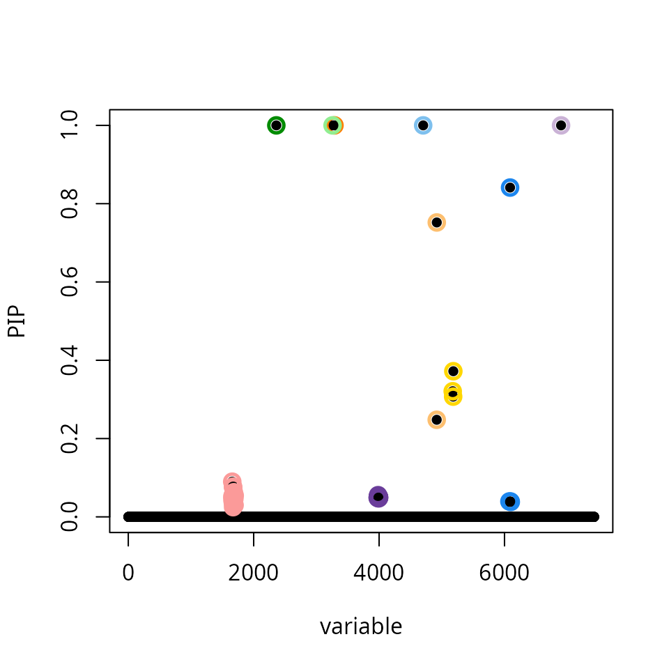
Another clue is that the fine-mapped SNPs explain >99% of the variation in gene expression, which might be explained by overfitting:
ypred <- predict(res_susie, X)
pve <- 1 - drop(res_susie$sigma2 / var(y))
round(100 * pve, 3)
# [1] 99.953
plot(y, ypred, pch = 20,
     xlab = "observed",
     ylab = "predicted")
abline(0, 1, col = "magenta", lty = "dotted")
SuSiE with Servin-Stephens SER
Setting estimate_residual_method = "NIG" switches SuSiE
to a variant of the single-effect regression (SER) model that accounts
for uncertainty in the residual variance. This is based on the linear
regression model for single-SNP association tests described in Servin and Stephens
(2007).
res_susie_small <-
  susie(X,y,L = 1,estimate_residual_method = "NIG",
        verbose = TRUE)
res_susie_small$sets$cs
# $L1
# [1] 4919 4920
This analysis looks more plausible as it identifies only 1 CS:
susie_plot(res_susie_small,y = "PIP")
And, indeed, the predictions with the Servin-Stephens SER do not seem to “overfit” the expression data quite so strongly.
pred_small <- predict(res_susie_small, X)
plot(y, ypred, pch = 20,col = "darkblue",
     xlab = "observed",
     ylab = "predicted")
points(y, pred_small, pch = 20, col = "darkorange")
abline(0, 1, col = "magenta", lty = "dotted")
legend("topleft", pch = c(20, 20), col = c("darkblue","darkorange"),
       legend = c("SuSiE (default Gaussian SER)",
                  "SuSiE (Servin-Stephens SER)"))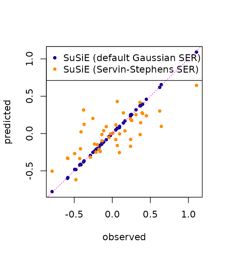
References
Servin, B. & Stephens, M. (2007). Imputation-based analysis of association studies: Candidate regions and quantitative traits. PLoS Genetics, 3(7): e114.
Denault et al (2025). Accounting for uncertainty in residual variances improves calibration for fine-mapping with small sample sizes. bioRxiv doi:10.1101/2025.05.16.654543.