Top-PC SuSiE versus fSuSiE

This vignette compares SuSiE on principal components (PCs) with fSuSiE. Running SuSiE on PCs is a natural way to reduce a functional response to one or a few scalar traits. The examples below show two cases. In the first example, PC 1 captures the simulated signal and identifies the causal SNP, but it does not estimate the region of the curve where the SNP acts. In the second example, SuSiE applied to the first principal component misses signals because different PCs capture different functional effects.

library(fsusieR)
library(susieR)
library(ggplot2)
library(cowplot)
library(reshape2)

Example 1: one functional effect

This is the same simulation used in the SuSiE limitation vignette. The effect of one SNP is a cosine function that spans multiple CpGs.

set.seed(1)
data(N3finemapping, package = "susieR")

X_full <- N3finemapping$X[seq_len(100), ]
T_m <- 128L

effect <- 1.2 * cos(seq_len(T_m) / T_m * 3 * pi)
effect[effect < 0] <- 0
effect[seq_len(40)] <- 0

true_pos <- 700L
y <- matrix(0, nrow = 100L, ncol = T_m)
for (i in seq_len(100L)) {
  y[i, ] <- X_full[i, true_pos] * effect + rnorm(T_m)
}

keep <- which(apply(X_full, 2, var) > 0)
X <- X_full[, keep]
true_pos_filt <- which(keep == true_pos)

plot(effect, pch = 19, xlab = "CpG", ylab = "effect")

Project the response matrix onto the top PCs and run SuSiE on each PC score.

pca_res <- prcomp(y, center = TRUE, scale. = TRUE)
pve <- pca_res$sdev^2 / sum(pca_res$sdev^2)

pc_results <- data.frame(
  PC = seq_len(5L),
  variance_explained = pve[seq_len(5L)],
  pip_at_true_snp = NA_real_,
  n_cs = NA_integer_,
  lead_snp_original = NA_integer_,
  lead_pip = NA_real_
)

for (pc in seq_len(5L)) {
  fit_pc <- susie(X, pca_res$x[, pc], L = 1L)
  pc_results$pip_at_true_snp[pc] <- fit_pc$pip[true_pos_filt]
  pc_results$n_cs[pc] <- length(fit_pc$sets$cs)
  pc_results$lead_snp_original[pc] <- keep[which.max(fit_pc$pip)]
  pc_results$lead_pip[pc] <- max(fit_pc$pip)
}

knitr::kable(pc_results, digits = 4)

PC	variance_explained	pip_at_true_snp	n_cs	lead_snp_original	lead_pip
1	0.0458	1.0000	1	700	1.0000
2	0.0331	0.0004	0	61	0.0969
3	0.0310	0.0011	0	756	0.0052
4	0.0296	0.0005	0	237	0.0382
5	0.0287	0.0000	0	1	0.0000

PC 1 captures the trait-driven direction cleanly and SuSiE on the PC 1 score returns a single, high-PIP credible set on the true SNP. That fixes the per-position-SuSiE recall problem: collapsing to one scalar derived from the curve gives a coherent fine-mapping signal. But PCA discards the per-position effect direction. The fit tells us a signal exists at one variant; it does not tell us where on the curve that variant acts. That target information is what fSuSiE preserves and PCA loses.

fit_one <- NULL
invisible(capture.output({
  fit_one <- susiF(y, X, L = 1L, post_processing = "TI", verbose = FALSE)
}))

fit_one$cs
fit_one$pip[true_pos_filt]
#> [[1]]
#> [1] 691
#> 
#> [1] 1

df_one_pip <- data.frame(snp = keep, pip = fit_one$pip)
P_one_pip <- ggplot(df_one_pip, aes(x = snp, y = pip)) +
  geom_point(color = "grey55", size = 0.8) +
  geom_vline(xintercept = true_pos, linetype = "dashed",
             color = "firebrick", alpha = 0.7) +
  geom_point(data = df_one_pip[df_one_pip$snp == true_pos, , drop = FALSE],
             color = "firebrick", size = 2.3) +
  coord_cartesian(ylim = c(0, 1)) +
  labs(x = "SNP original index", y = "PIP", title = "fSuSiE PIPs") +
  theme_classic()

df_one_curve <- data.frame(
  position = seq_along(fit_one$fitted_func[[1]]),
  estimate = fit_one$fitted_func[[1]],
  upper = fit_one$cred_band[[1]][1, ],
  lower = fit_one$cred_band[[1]][2, ],
  truth = effect
)

P_one_effect <- ggplot(df_one_curve, aes(x = position)) +
  geom_ribbon(aes(ymin = lower, ymax = upper), fill = "skyblue",
              alpha = 0.45) +
  geom_point(aes(y = truth), color = "grey30", size = 1.1) +
  geom_line(aes(y = estimate), color = "firebrick", linewidth = 1) +
  geom_hline(yintercept = 0, linetype = "dotted", color = "grey50") +
  labs(x = "CpG", y = "effect", title = "fSuSiE recovered effect curve") +
  theme_classic()

plot_grid(P_one_pip, P_one_effect, nrow = 1L, rel_widths = c(1, 1.25))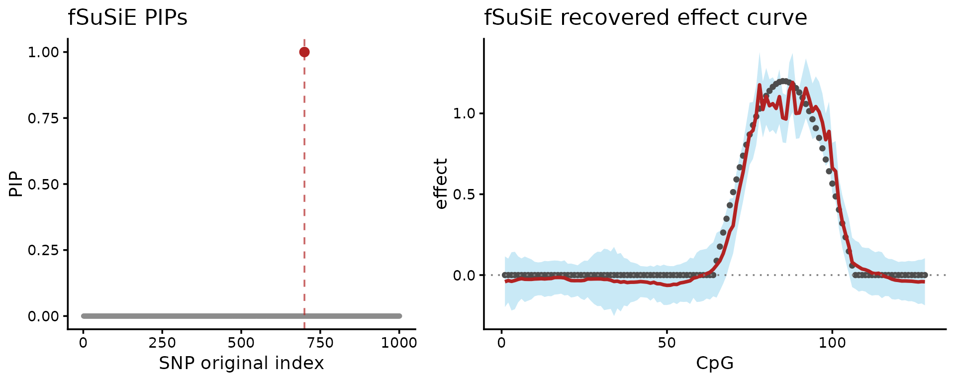

These plots show two results: on the left-hand side, the fine-mapping signal (PIPs); on the right-hand side, the estimated effect on the methylation levels (red = posterior mean, light blue = credible bands).

Example 2: multiple functional effects

We next regenerate the toy methylation example. The methylation levels of 100 individuals are measured at 32 CpGs. Among the 12 candidate SNPs, 3 SNPs affect the methylation levels: 2 SNPs affect the same cluster of 8 CpGs, and the other SNP affects a different cluster of 8 CpGs.

set.seed(1)
n <- 100
m <- 32
p <- 12

cs_colors <- c("dodgerblue", "darkorange", "red")

maf <- 0.05 + 0.45 * runif(p)
snpids <- paste0("SNP-", seq_len(p))
cpgids <- paste0("CpG-", seq_len(m))

X <- (runif(n * p) < maf) + (runif(n * p) < maf)
X <- matrix(X, n, p, byrow = TRUE)
storage.mode(X) <- "double"
X[, 4] <- X[, 3] + 0.03 * rnorm(n)
colnames(X) <- snpids

F <- matrix(0, p, m)
F[1, 9:16] <- 2.3
F[9, 9:16] <- -2.3
F[3, 25:32] <- 2
rownames(F) <- snpids
colnames(F) <- cpgids

E <- matrix(3 * rnorm(n * m), n, m)
Y <- X %*% F + E
baseline <- min(Y)
Y <- Y - baseline

x <- X[, 3]
pdat <- data.frame(
  cpg = rep(seq_len(m), each = n) + runif(m * n, min = -0.2, max = 0.2),
  meth_level = as.vector(Y),
  geno = factor(rep(x, times = m))
)
pdat_lines <- data.frame(
  cpg = rep(seq_len(m), times = 3),
  geno = factor(rep(0:2, each = m)),
  meth_level = rep(c(rep(0, 8), rep(-0.75, 8), rep(0, 16)), times = 3)
)
pdat_lines$meth_level <- pdat_lines$meth_level - baseline
rows <- with(pdat_lines, geno == 1 & cpg > 24)
pdat_lines[rows, "meth_level"] <- pdat_lines[rows, "meth_level"] + 2
rows <- with(pdat_lines, geno == 2 & cpg > 24)
pdat_lines[rows, "meth_level"] <- pdat_lines[rows, "meth_level"] + 4

ggplot(pdat, aes(x = cpg, y = meth_level, color = geno)) +
  geom_point(shape = 20, size = 1.25) +
  scale_x_continuous(breaks = c(0, seq(4, 32, 4))) +
  scale_color_manual(values = c("darkblue", "limegreen", "darkorange")) +
  geom_line(data = pdat_lines,
            aes(x = cpg, y = meth_level, group = geno),
            color = "black", linewidth = 1.9) +
  geom_line(data = pdat_lines, linewidth = 1.25) +
  labs(x = "CpG", y = "methylation level", color = "genotype") +
  theme_cowplot(font_size = 11)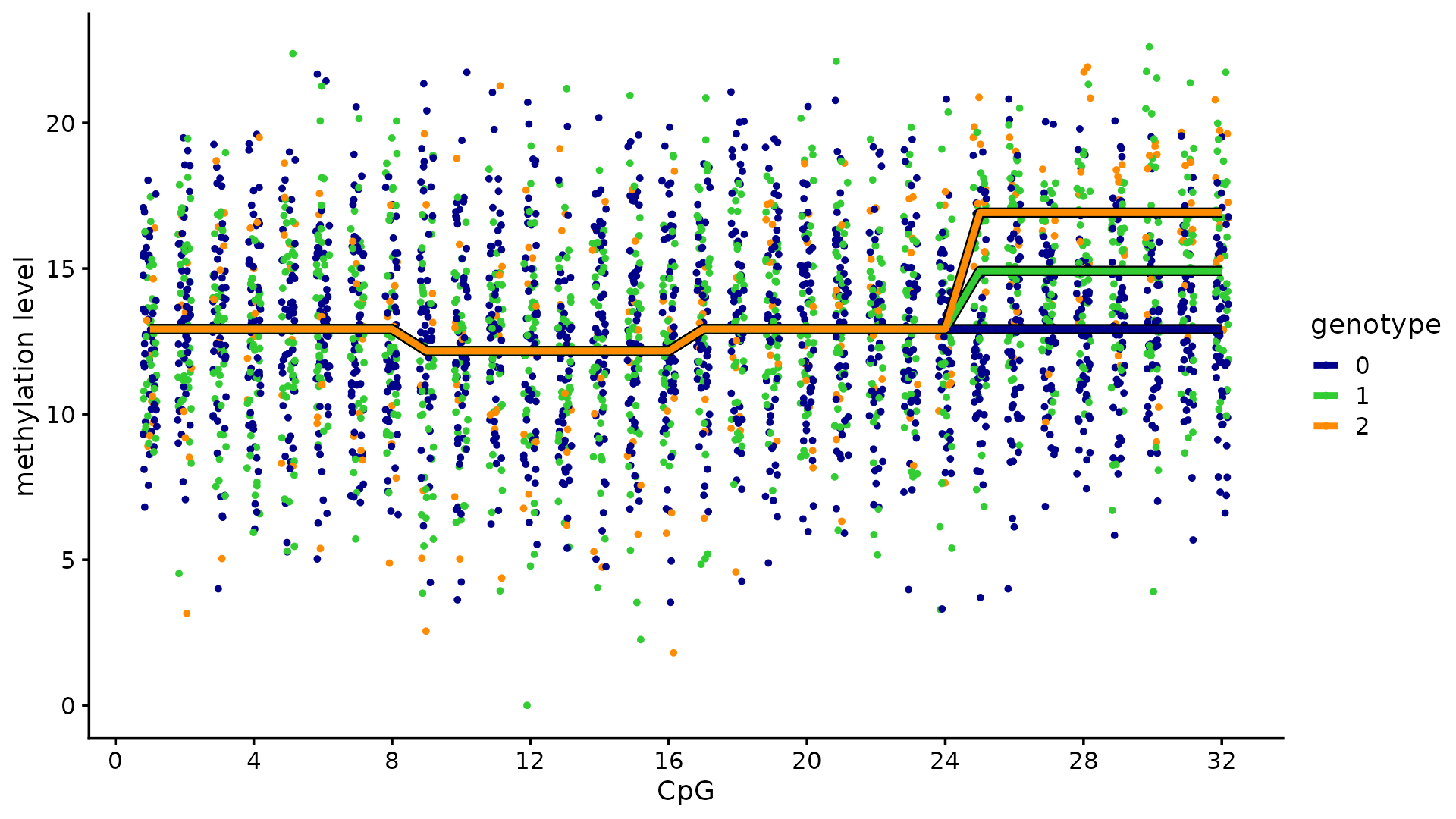

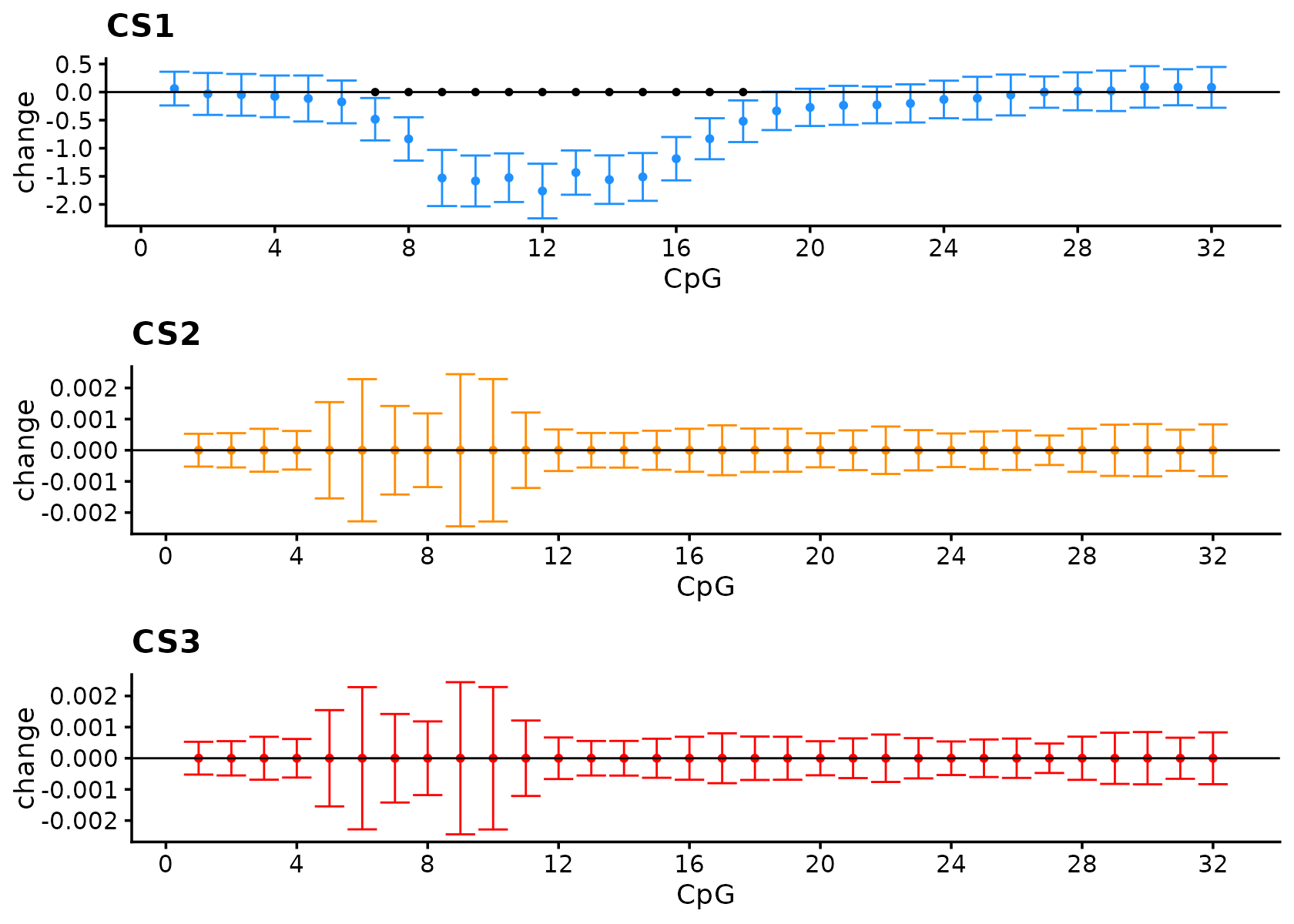
fSuSiE correctly selects the causal SNPs and outputs estimates that reflect the effect of the SNP.

fit_multi <- NULL
invisible(capture.output({
  fit_multi <- susiF(
    Y, X, L = 3, filter_cs = FALSE, prior = "mixture_normal",
    post_processing = "TI", verbose = FALSE
  )
}))

fit_multi$cs
#> [[1]]
#> SNP-9 
#>     9 
#> 
#> [[2]]
#> SNP-3 SNP-4 
#>     3     4 
#> 
#> [[3]]
#> SNP-1 
#>     1

Visualize the effect.

out <- lapply(seq_len(3L), function(i) {
  get_fitted_effect(fit_multi, l = i, cred_band = TRUE, alpha = 0.05)
})

effect_plot <- function(i) {
  pdat <- data.frame(
    cpg = seq_len(m),
    estimate = out[[i]]$effect,
    lower = out[[i]]$cred_band["low", ],
    upper = out[[i]]$cred_band["up", ]
  )
  rows <- with(pdat, which(lower > 0 | upper < 0))
  pdat2 <- data.frame(cpg = rows, estimate = rep(0, length(rows)))
  ggplot(pdat, aes(x = cpg, y = estimate, ymin = lower, ymax = upper)) +
    geom_point(color = cs_colors[i], size = 1) +
    geom_errorbar(color = cs_colors[i], linewidth = 0.4) +
    geom_hline(yintercept = 0, color = "black", linewidth = 0.4) +
    geom_point(data = pdat2, mapping = aes(x = cpg, y = estimate),
               shape = 20, color = "black", size = 1.5,
               inherit.aes = FALSE) +
    scale_x_continuous(breaks = c(0, seq(4, 32, 4))) +
    labs(x = "CpG", y = "change", title = paste0("CS", i)) +
    theme_cowplot(font_size = 11)
}

plot_grid(
  effect_plot(1),
  effect_plot(2),
  effect_plot(3),
  nrow = 3L,
  ncol = 1L
)

Now run SuSiE on principal components. Here we use L = 1 to show what is captured by each individual PC score.

pca_multi <- prcomp(Y, center = TRUE, scale. = TRUE)
pve_multi <- pca_multi$sdev^2 / sum(pca_multi$sdev^2)
causal_snps <- c(1L, 3L, 9L)

pc_multi_results <- data.frame(
  PC = seq_len(5L),
  variance_explained = pve_multi[seq_len(5L)],
  pip_snp1 = NA_real_,
  pip_snp3 = NA_real_,
  pip_snp9 = NA_real_,
  n_cs = NA_integer_,
  lead_snp = NA_integer_,
  lead_pip = NA_real_
)

pc_multi_fits <- vector("list", 5L)
for (pc in seq_len(5L)) {
  fit_pc <- susie(X, pca_multi$x[, pc], L = 1L)
  pc_multi_fits[[pc]] <- fit_pc
  pc_multi_results$pip_snp1[pc] <- fit_pc$pip[1]
  pc_multi_results$pip_snp3[pc] <- fit_pc$pip[3]
  pc_multi_results$pip_snp9[pc] <- fit_pc$pip[9]
  pc_multi_results$n_cs[pc] <- length(fit_pc$sets$cs)
  pc_multi_results$lead_snp[pc] <- which.max(fit_pc$pip)
  pc_multi_results$lead_pip[pc] <- max(fit_pc$pip)
}

knitr::kable(pc_multi_results, digits = 4)

PC	variance_explained	pip_snp1	pip_snp3	pip_snp9	n_cs	lead_snp	lead_pip
1	0.1024	0.000	0.0000	1.0000	1	9	1.0000
2	0.0724	0.000	0.6087	0.0000	1	3	0.6087
3	0.0597	0.051	0.0302	0.0292	0	12	0.6715
4	0.0523	0.000	0.0000	0.0000	0	1	0.0000
5	0.0506	0.000	0.0000	0.0000	0	1	0.0000

Results on the first PC:

pc_multi_fits[[1]]$sets
#> $cs
#> $cs$L1
#> [1] 9
#> 
#> 
#> $purity
#>    min.abs.corr mean.abs.corr median.abs.corr
#> L1            1             1               1
#> 
#> $cs_index
#> [1] 1
#> 
#> $coverage
#> [1] 1
#> 
#> $requested_coverage
#> [1] 0.95

When running SuSiE on the second PC:

pc_multi_fits[[2]]$sets
#> $cs
#> $cs$L1
#> [1] 3 4
#> 
#> 
#> $purity
#>    min.abs.corr mean.abs.corr median.abs.corr
#> L1    0.9989364     0.9989364       0.9989364
#> 
#> $cs_index
#> [1] 1
#> 
#> $coverage
#> [1] 1
#> 
#> $requested_coverage
#> [1] 0.95

In this case, most of the variation in the data is due to orthogonal effects, and principal components are orthogonal by construction. The first PC captures the effect of one SNP and has no information about the other SNP, and vice versa. This is why SuSiE applied to only the top PC can miss signals.

William Denault, Peter Carbonetto and Gao Wang

2026-05-13

Example 1: one functional effect

Example 2: multiple functional effects