Implementation of the SuSiF method.
Usage
susiF(
  Y,
  X,
  L = 2,
  pos = NULL,
  prior = c("mixture_normal", "mixture_normal_per_scale"),
  verbose = TRUE,
  maxit = 100,
  tol = 1e-06,
  cov_lev = 0.95,
  min_purity = 0.5,
  filter_cs = TRUE,
  init_pi0_w = 1,
  nullweight = 0.01,
  control_mixsqp = list(verbose = FALSE, eps = 1e-06, numiter.em = 40),
  thresh_lowcount = 0,
  cal_obj = FALSE,
  L_start = 3,
  quantile_trans = FALSE,
  greedy = TRUE,
  backfit = TRUE,
  gridmult = sqrt(2),
  max_scale = 10,
  max_SNP_EM = 100,
  max_step_EM = 1,
  cor_small = FALSE,
  filter.number = 10,
  family = "DaubLeAsymm",
  post_processing = c("smash", "TI", "HMM", "none"),
  e = 0.001,
  tol_null_prior = 0.001,
  lbf_min = 0.1
)
Arguments
- Y
functional phenotype, matrix of size N by size J. The underlying algorithm uses wavelet, which assumes that J is of the form J^2. If J is not a power of 2, susiF internally remaps the data into a grid of length 2^J
- X
matrix of size n by p contains the covariates
- L
upper bound on the number of effects to fit (if not specified, set to =2)
- pos
vector of length J, corresponding to position/time pf the observed column in Y, if missing, suppose that the observation are evenly spaced
- prior
specify the prior used in susiF. The two available choices are available "mixture_normal_per_scale", "mixture_normal". Default "mixture_normal_per_scale", if this susiF is too slow, consider using "mixture_normal" using "mixture_normal" which is up to 40% faster but may lead to slight power loss
- verbose
If
verbose = TRUE, the algorithm's progress, and a summary of the optimization settings are printed on the console.- maxit
Maximum number of IBSS iterations.
- tol
a small, non-negative number specifying the convergence tolerance for the IBSS fitting procedure. The fitting procedure will halt when the difference in the variational lower bound or “ELBO” (the objective function to be maximized), is less than
tol.- cov_lev
numeric between 0 and 1, corresponding to the expected level of coverage of the CS if not specified, set to 0.95
- min_purity
minimum purity for estimated credible sets
- filter_cs
logical, if TRUE filters the credible set (removing low-purity) cs and cs with estimated prior equal to 0). Set as TRUE by default.
- init_pi0_w
starting value of weight on null component in mixsqp (between 0 and 1)
- nullweight
numeric value for penalizing likelihood at point mass 0. This number roughly corresponds to the number of zeros observation you add (useful in small sample size). Default is 10 as recommended by Stephens in False discovery rate a new deal. Setting it too low tend lead to adding false discoveries. Setting it too high may reduce power.
- control_mixsqp
list of parameter for mixsqp function see mixsqp package
- thresh_lowcount
numeric, used to check the wavelet coefficients have problematic distribution (very low dispersion even after standardization). Basically, check if the median of the absolute value of the distribution of a wavelet coefficient is below this threshold. If yes, the algorithm discards this wavelet coefficient (setting its estimate effect to 0 and estimate sd to 1). Set to 0 by default. It can be useful when analyzing sparse data from sequence based assay or small samples.
- cal_obj
logical if set as TRUE compute ELBO for convergence monitoring
- L_start
number of effect initialized at the start of the algorithm
- quantile_trans
logical, if set as TRUE perform normal quantile, transform on wavelet coefficients
- greedy
logical, if TRUE allows greedy search for extra effect (up to L specified by the user). Set as TRUE by default
- backfit
logical, if TRUE, allow discarding effect via back fitting. Set as true by default as TRUE. We advise keeping it as TRUE.
- gridmult
numeric used to control the number of components used in the mixture prior (see ashr package for more details). From the ash function: multiplier by which the default grid values for mixed differ from one another. (Smaller values produce finer grids.). Increasing this value may reduce computational time.
- max_scale
numeric, define the maximum of wavelet coefficients used in the analysis (2^max_scale). Set 10 true by default.
- max_SNP_EM
maximum number of SNP used for learning the prior. By default, set to 1000. Reducing this may help reduce the computational time. We advise to keep it at least larger than 50
- max_step_EM
max_step_EM
- cor_small
logical set to FALSE by default. If TRUE used the Bayes factor from Valen E Johnson JRSSB 2005 instead of Wakefield approximation for Gen Epi 2009 The Bayes factor from Valen E Johnson JRSSB 2005 tends to have better coverage in small sample sizes. We advise using this parameter if n<50
- filter.number
see documentation of wd from wavethresh package
- family
see documentation of wd from wavethresh package
- post_processing
character, use "TI" for translation invariant wavelet estimates, "HMM" for hidden Markov model (useful for estimating non-zero regions), "none" for simple wavelet estimate (not recommended) and "smashr" experimental. In general we recommend using TI as post processing, Nonetheless the HMM perform particularly well when analysing data with say few sampling points (i.e ncol(Y)<30) or when the data are particularly noisy (low signal noise ratio). However, we found that the HMM post processing is quite sensitive to the Gaussian assumption and we advise to use data transformation if your data are not normally distributed, e.g., using log1p( Y[i,]/si) for count data data where si is the individual scaling factor as defined in $s_i = _j=1^p Y_ij 1n_i=1^n_j=1^p Y_ij$ or using M-value instead of Beta value when analysing DNA methylation data. The option smashr is experimental and tend to give good point estimate but the credible band can be to narrow and so should be used with caution.
- e
threshold value is used to avoid computing posteriors that have low alpha values. Set it to 0 to compute the entire posterior. default value is 0.001
- tol_null_prior
threshold to consider prior to be null. If the estimated weight on the point mass at zero is larger than 1-tol_null_prior then set prior weight on point mass to be 1. In the mixture normal this corresponds to removing the effect. In the mixutre per scale prior this corresponds to setting the prior of a given scale to at point mass at 0.
- lbf_min
numeric discard low purity cs in the IBSS fitting procedure if the largest log Bayes factors is lower than this value
Value
A "susiF" object with some or all of the following
elements:
- alpha
List of length L containing the posterior inclusion probabilities for each effect.
- pip
Vector of length J, containing the posterior inclusion probability for each covariate.
- cs
List of length L. Each element is the credible set of the lth effect.
- purity
List of length L. Each element is the purity of the lth effect.
- fitted_func
List of length L. Each element is a vector of length J containing the Lth estimated single effect.
- cred_band
List of length L. Each element is a list of length J, containing the credible band of the Lth effect at each position
- sigma2
The estimated residual variance.
- lBF
List of length L containing the log-Bayes factor for each effect.
- ind_fitted_func
Matrix of the individual estimated genotype effect.
- outing_grid
The grid on which the effects are estimated. Ssee the introductory vignette for more details.
- runtime
runtime of the algorithm
- G_prior
A list of of ash objects containing the prior mixture component.
- est_pi
List of length L. Each element contains the estimated prior mixture weights for each effect.
- est_sd
Ehe estimated prior mixture for each effect.
- ELBO
The ELBO value at each iteration of the algorithm.
- fitted_wc
List of length L. Each element is a matrix containing the conditional wavelet coefficients (first moment) for a single effect. For internal use only. The results in
fitted_funcwill correspond to this wavelet coefficient ifpost_processing = "none"(which is not recommended).- fitted_wc2
List of length L. Each element is a matrix containing the conditional wavelet coefficients (second-moment) for a single effect.
Examples
library(fsusieR)
set.seed(1)
#Example using curves simulated under the Mixture normal per scale prior
rsnr <- 0.2 #expected root signal noise ratio
N <- 100 #Number of individuals
P <- 100 #Number of covariates/SNP
pos1 <- 1 #Position of the causal covariate for effect 1
pos2 <- 5 #Position of the causal covariate for effect 2
lev_res <- 7#length of the molecular phenotype (2^lev_res)
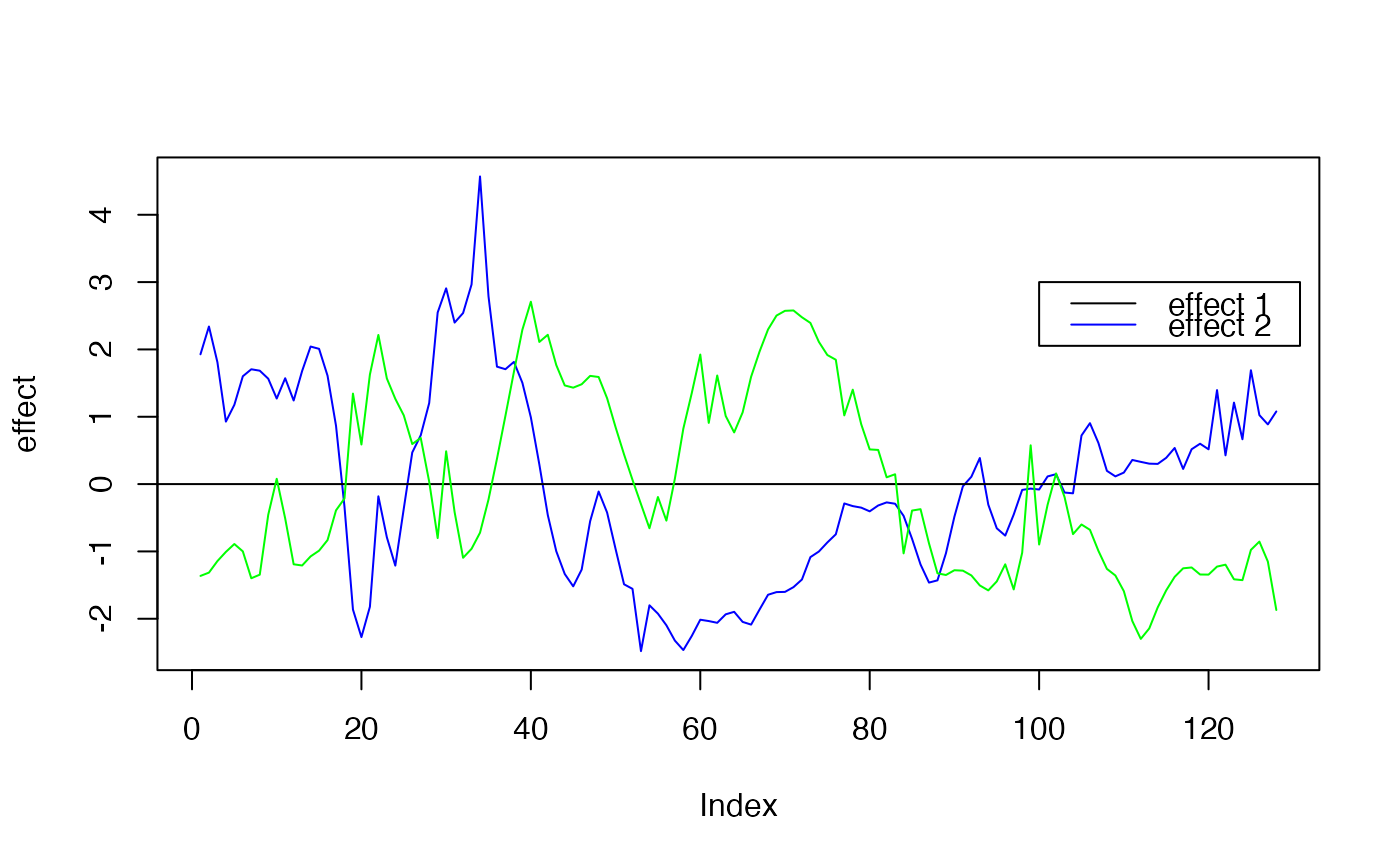
f1 <- simu_IBSS_per_level(lev_res )$sim_func#first effect
f2 <- simu_IBSS_per_level(lev_res )$sim_func #second effect
plot( f1, type ="l", ylab="effect", col="blue")
abline(a=0,b=0)
lines(f2, type="l", col="green")
legend(x=100,
y=3,
lty = rep(1,3),
legend= c("effect 1", "effect 2" ),
col=c("black","blue","yellow"))
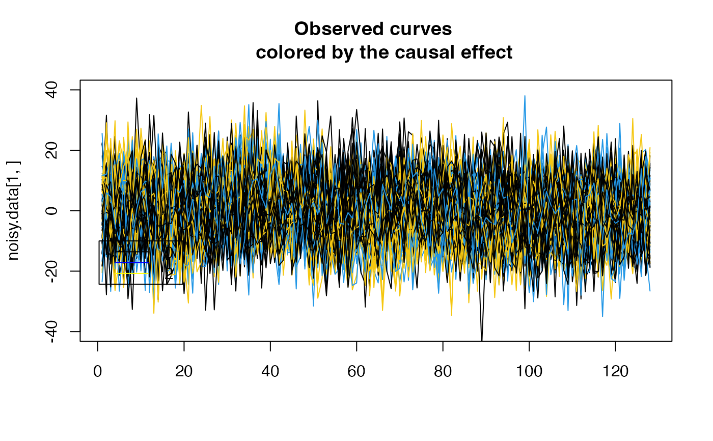
 G = matrix(sample(c(0, 1,2), size=N*P, replace=TRUE), nrow=N, ncol=P) #Genotype
beta0 <- 0
beta1 <- 1
beta2 <- 1
noisy.data <- list()
for ( i in 1:N)
{
f1_obs <- f1
f2_obs <- f2
noise <- rnorm(length(f1), sd= (1/ rsnr ) * var(f1))
noisy.data [[i]] <- beta1*G[i,pos1]*f1_obs + beta2*G[i,pos2]*f2_obs + noise
}
noisy.data <- do.call(rbind, noisy.data)
plot( noisy.data[1,], type = "l", col=(G[1, pos1]*3+1),
main ="Observed curves \n colored by the causal effect" , ylim= c(-40,40), xlab="")
for ( i in 2:N)
{
lines( noisy.data[i,], type = "l", col=(G[i, pos1]*3+1))
}
legend(x=0.3,
y=-10,
lty = rep(1,3),
legend= c("0", "1","2"),
col=c("black","blue","yellow"))
G = matrix(sample(c(0, 1,2), size=N*P, replace=TRUE), nrow=N, ncol=P) #Genotype
beta0 <- 0
beta1 <- 1
beta2 <- 1
noisy.data <- list()
for ( i in 1:N)
{
f1_obs <- f1
f2_obs <- f2
noise <- rnorm(length(f1), sd= (1/ rsnr ) * var(f1))
noisy.data [[i]] <- beta1*G[i,pos1]*f1_obs + beta2*G[i,pos2]*f2_obs + noise
}
noisy.data <- do.call(rbind, noisy.data)
plot( noisy.data[1,], type = "l", col=(G[1, pos1]*3+1),
main ="Observed curves \n colored by the causal effect" , ylim= c(-40,40), xlab="")
for ( i in 2:N)
{
lines( noisy.data[i,], type = "l", col=(G[i, pos1]*3+1))
}
legend(x=0.3,
y=-10,
lty = rep(1,3),
legend= c("0", "1","2"),
col=c("black","blue","yellow"))
 Y <- noisy.data
X <- G
#Running fSuSiE
out <- susiF(Y,X,L=2 , prior = 'mixture_normal_per_scale')
#> [1] "Scaling columns of X and Y to have unit variance"
#> [1] "Starting initialization"
#> [1] "Data transform"
#> [1] "Discarding 0 wavelet coefficients out of 128"
#> [1] "Data transform done"
#> [1] "Initializing prior"
#> [1] "Initialization done"
#> [1] "Fitting effect 1 , iter 1"
#> [1] "Fitting effect 2 , iter 1"
#> [1] "Discarding 0 effects"
#> [1] "Greedy search and backfitting done"
#> [1] "Fitting effect 1 , iter 2"
#> [1] "Fitting effect 2 , iter 2"
#> [1] "Fine mapping done, refining effect estimates using cylce spinning wavelet transform"
plot_susiF(out)
#> $pip
Y <- noisy.data
X <- G
#Running fSuSiE
out <- susiF(Y,X,L=2 , prior = 'mixture_normal_per_scale')
#> [1] "Scaling columns of X and Y to have unit variance"
#> [1] "Starting initialization"
#> [1] "Data transform"
#> [1] "Discarding 0 wavelet coefficients out of 128"
#> [1] "Data transform done"
#> [1] "Initializing prior"
#> [1] "Initialization done"
#> [1] "Fitting effect 1 , iter 1"
#> [1] "Fitting effect 2 , iter 1"
#> [1] "Discarding 0 effects"
#> [1] "Greedy search and backfitting done"
#> [1] "Fitting effect 1 , iter 2"
#> [1] "Fitting effect 2 , iter 2"
#> [1] "Fine mapping done, refining effect estimates using cylce spinning wavelet transform"
plot_susiF(out)
#> $pip
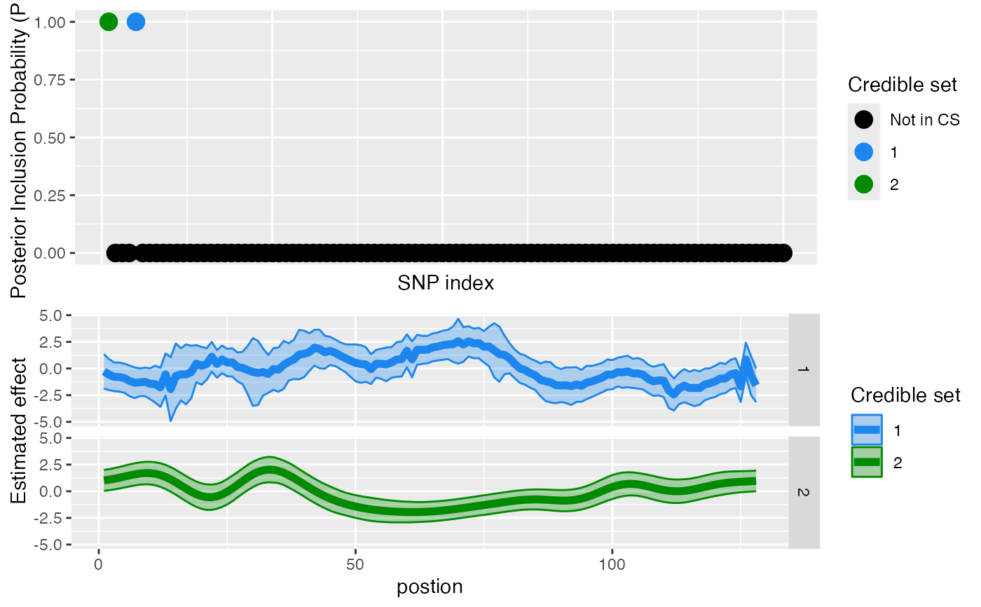 #>
#> $effect
#>
#> $effect
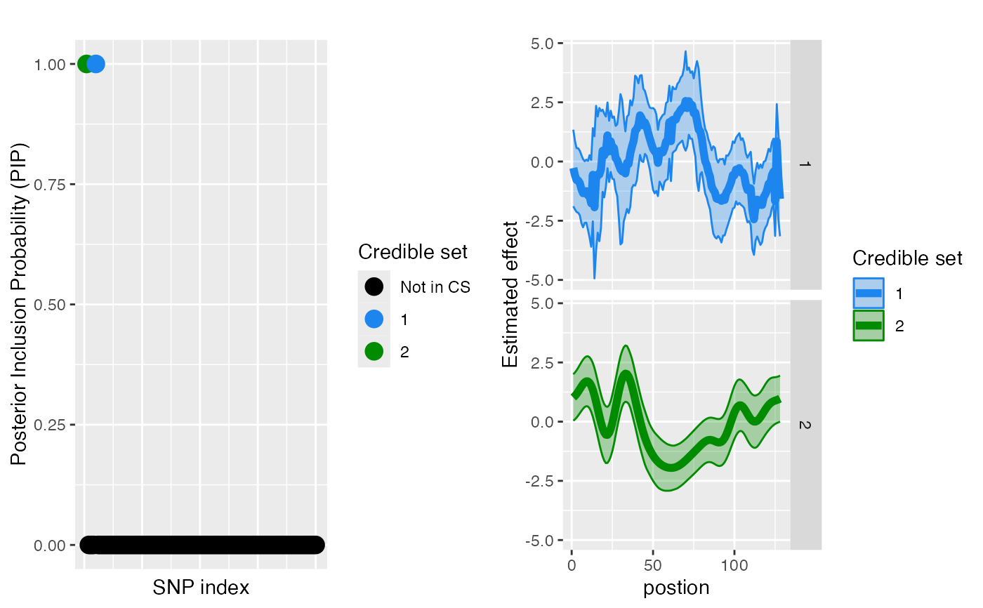 #>
#### Find out which regions are affected by the different CS
affected_reg(obj = out)
#> CS Start End
#> 1 1 2 12
#> 2 1 14 14
#> 7 1 38 49
#> 8 1 58 78
#> 3 1 85 102
#> 4 1 107 108
#> 5 1 111 112
#> 6 1 115 124
#> 10 2 1 14
#> 11 2 28 38
#> 9 2 48 92
#> 12 2 123 125
#> 13 2 127 128
# This corresponds to the regions where the credible bands are
# "crossing zero"/i.e. the effects are likely not to be 0 in this
# region.
#
# You can also access the information directly in the output of
# susiF as follows.
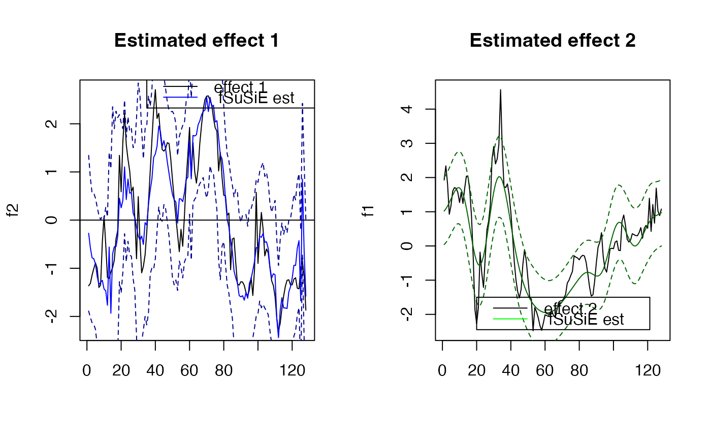
par(mfrow=c(1,2))
plot( f2, type="l", main="Estimated effect 1", xlab="")
lines(unlist(out$fitted_func[[1]]),col='blue' )
lines(unlist(out$cred_band[[1]][1,]),col='darkblue',lty=2 )
lines(unlist(out$cred_band[[1]][2,]),col='darkblue' ,lty=2 )
abline(a=0,b=0)
legend(x= 35,
y=3,
lty= rep(1,2),
legend = c("effect 1"," fSuSiE est "),
col=c("black","blue" )
)
plot( f1, type="l", main="Estimated effect 2", xlab="")
lines(unlist(out$fitted_func[[2]]),col='darkgreen' )
lines(unlist(out$cred_band[[2]][1,]),col='darkgreen',lty=2 )
lines(unlist(out$cred_band[[2]][2,]),col='darkgreen' ,lty=2 )
#'abline(a=0,b=0)
legend(x= 20,
y=-1.5,
lty= rep(1,2),
legend = c("effect 2"," fSuSiE est "),
col=c("black","green" )
)
#>
#### Find out which regions are affected by the different CS
affected_reg(obj = out)
#> CS Start End
#> 1 1 2 12
#> 2 1 14 14
#> 7 1 38 49
#> 8 1 58 78
#> 3 1 85 102
#> 4 1 107 108
#> 5 1 111 112
#> 6 1 115 124
#> 10 2 1 14
#> 11 2 28 38
#> 9 2 48 92
#> 12 2 123 125
#> 13 2 127 128
# This corresponds to the regions where the credible bands are
# "crossing zero"/i.e. the effects are likely not to be 0 in this
# region.
#
# You can also access the information directly in the output of
# susiF as follows.
par(mfrow=c(1,2))
plot( f2, type="l", main="Estimated effect 1", xlab="")
lines(unlist(out$fitted_func[[1]]),col='blue' )
lines(unlist(out$cred_band[[1]][1,]),col='darkblue',lty=2 )
lines(unlist(out$cred_band[[1]][2,]),col='darkblue' ,lty=2 )
abline(a=0,b=0)
legend(x= 35,
y=3,
lty= rep(1,2),
legend = c("effect 1"," fSuSiE est "),
col=c("black","blue" )
)
plot( f1, type="l", main="Estimated effect 2", xlab="")
lines(unlist(out$fitted_func[[2]]),col='darkgreen' )
lines(unlist(out$cred_band[[2]][1,]),col='darkgreen',lty=2 )
lines(unlist(out$cred_band[[2]][2,]),col='darkgreen' ,lty=2 )
#'abline(a=0,b=0)
legend(x= 20,
y=-1.5,
lty= rep(1,2),
legend = c("effect 2"," fSuSiE est "),
col=c("black","green" )
)
 par(mfrow=c(1,1))