Key ideas for molecular profile QTL fine-mapping with applications to DNAm QTL
William Denault and Peter Carbonetto
2026-02-11
Source:vignettes/susie_top_PC_fails.Rmd
susie_top_PC_fails.RmdIn this vignette we illustrate some of the key ideas underlying fSuSiE by applying fSuSiE to analyze a toy methylation data set.
Set the seed so that the results can be reproduced.
set.seed(1)IN this vignette we showcase a simulation example where SuSiE applied to the first principal component misses signals. We regenerate the example from the methyl_demo.
Simulate data
We simulate a “toy” methylation data set in which the methylation levels of 100 individuals are measured at 32 CpGs.
Among the 12 candidate SNPs, 3 SNPs affect the methylation levels: 2 SNPs affect the methylation levels of the same cluster of 8 CpGs, and the other SNP affects the methylation levels of different cluster of 8 CpGs.
n <- 100
m <- 32
p <- 12

cs_colors <- c("dodgerblue","darkorange","red")

maf <- 0.05 + 0.45*runif(p)

snpids <- paste0("SNP-",1:p)
cpgids <- paste0("CpG-",1:m)

X <- (runif(n*p) < maf) +
  (runif(n*p) < maf)
X <- matrix(X,n,p,byrow = TRUE)
storage.mode(X) <- "double"
X[,4] <- X[,3] + 0.03*rnorm(n)
colnames(X) <- snpids

F <- matrix(0,p,m)
F[1,9:16] <- 2.3
F[9,9:16] <- (-2.3)
F[3,25:32] <- 2
rownames(F) <- snpids
colnames(F) <- cpgids

E <- matrix(3*rnorm(n*m),n,m)
Y <- X %*% F
Y <- Y + E
baseline <- min(Y)
Y <- Y - baseline

pdat <- melt(Y)
x    <- X[,3]
pdat <- data.frame(cpg        = rep(1:m,each = n) +
                     runif(m*n,min = -0.2,max = 0.2),
                   meth_level = as.vector(Y),
                   geno       = factor(x))
pdat_lines <- data.frame(cpg = rep(1:m,times = 3),
                         geno = factor(rep(0:2,each = m)),
                         meth_level = rep(c(rep(0,8),rep(-0.75,8),rep(0,16)),
                                          times = 3))
pdat_lines$meth_level <- pdat_lines$meth_level - baseline
rows <- which(with(pdat_lines,geno == 1 & cpg > 24))
pdat_lines[rows,"meth_level"] <- pdat_lines[rows,"meth_level"] + 2
rows <- which(with(pdat_lines,geno == 2 & cpg > 24))
pdat_lines[rows,"meth_level"] <- pdat_lines[rows,"meth_level"] + 4
p1 <- ggplot(pdat, aes(x = cpg, y = meth_level, color = geno)) +
  geom_point(shape = 20, size = 1.25) +
  scale_x_continuous(breaks = c(0, seq(4, 32, 4))) +
  scale_color_manual(values = c("darkblue", "limegreen", "darkorange")) +
  geom_line(data = pdat_lines, aes(x = cpg, y = meth_level, group = geno),
            color = "black", size = 1.9) +  # Black line for contrast
  geom_line(data = pdat_lines, size = 1.25) +  # Original colored lines
  labs(x = "CpG", y = "methylation level", color = "genotype") +
  theme_cowplot(font_size = 11)
# Warning: Using `size` aesthetic for lines was deprecated in ggplot2 3.4.0.
# ℹ Please use `linewidth` instead.
# This warning is displayed once per session.
# Call `lifecycle::last_lifecycle_warnings()` to see where this warning was
# generated.
print(p1)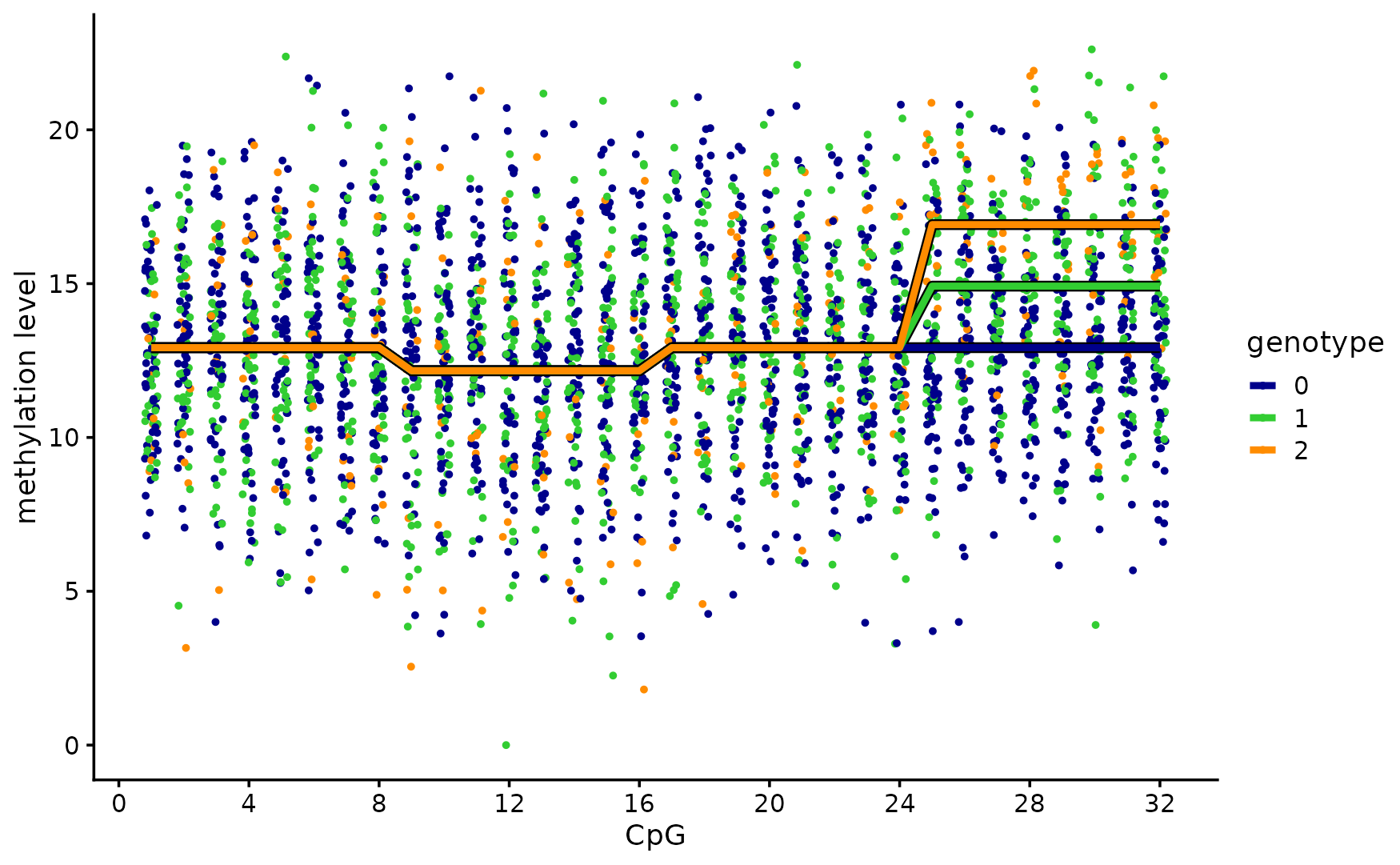
As showm in the previous vignette fsusie correctly selection the causal SNP and outputs estiamtes that reflect the effect of the SNP
fit_TI <- susiF(Y,X,L = 3,filter_cs = FALSE,prior = "mixture_normal" )

fit_TI$cs
# [1] "Scaling columns of X and Y to have unit variance"
# [1] "Starting initialization"
# [1] "Data transform"
# [1] "Discarding  0 wavelet coefficients out of  32"
# [1] "Data transform done"
# [1] "Initializing prior"
# [1] "Initialization done"
# [1] "Fitting effect  1 , iter 1"
# [1] "Fitting effect  2 , iter 1"
# [1] "Fitting effect  3 , iter 1"
# [1] "Discarding  0  effects"
# [1] "Greedy search and backfitting done"
# [1] "Fitting effect  1 , iter 2"
# [1] "Fitting effect  2 , iter 2"
# [1] "Fitting effect  3 , iter 2"
# [1] "Fitting effect  1 , iter 3"
# [1] "Fitting effect  2 , iter 3"
# [1] "Fitting effect  3 , iter 3"
# [1] "Fine mapping done, refining effect estimates using cylce spinning wavelet transform"
# [[1]]
# SNP-9
#     9
#
# [[2]]
# SNP-3 SNP-4
#     3     4
#
# [[3]]
# SNP-1
#     1
Visualize the effect
out <- lapply(1:3,function (i) get_fitted_effect(fit_TI,l = i,cred_band = TRUE,
                                                 alpha = 0.05))
effect_plot <- function (i) {
  pdat <- data.frame(cpg      = 1:m,
                     estimate = out[[i]]$effect,
                     lower    = out[[i]]$cred_band["low",],
                     upper    = out[[i]]$cred_band["up",])
  rows <- with(pdat,which(lower > 0 | upper < 0))
  pdat2 <- data.frame(cpg = rows,estimate = 0)
  return(ggplot(pdat,aes(x = cpg,y = estimate,ymin = lower,ymax = upper)) +
         geom_point(color = cs_colors[i],size = 1) +
         geom_errorbar(color = cs_colors[i],linewidth = 0.4) +
         geom_hline(yintercept = 0,color = "black",linewidth = 0.4) +
         geom_point(data = pdat2,mapping = aes(x = cpg,y = estimate),
                    shape = 20,color = "black",size = 1.5,
                    inherit.aes = FALSE) +
         scale_x_continuous(breaks = c(0,seq(4,32,4))) +
         labs(x = "CpG",y = "change",title = paste0("CS",i)) +
         theme_cowplot(font_size = 11))
}
plot_grid(effect_plot(1),
          effect_plot(2),
          effect_plot(3),
nrow = 3,ncol = 1) 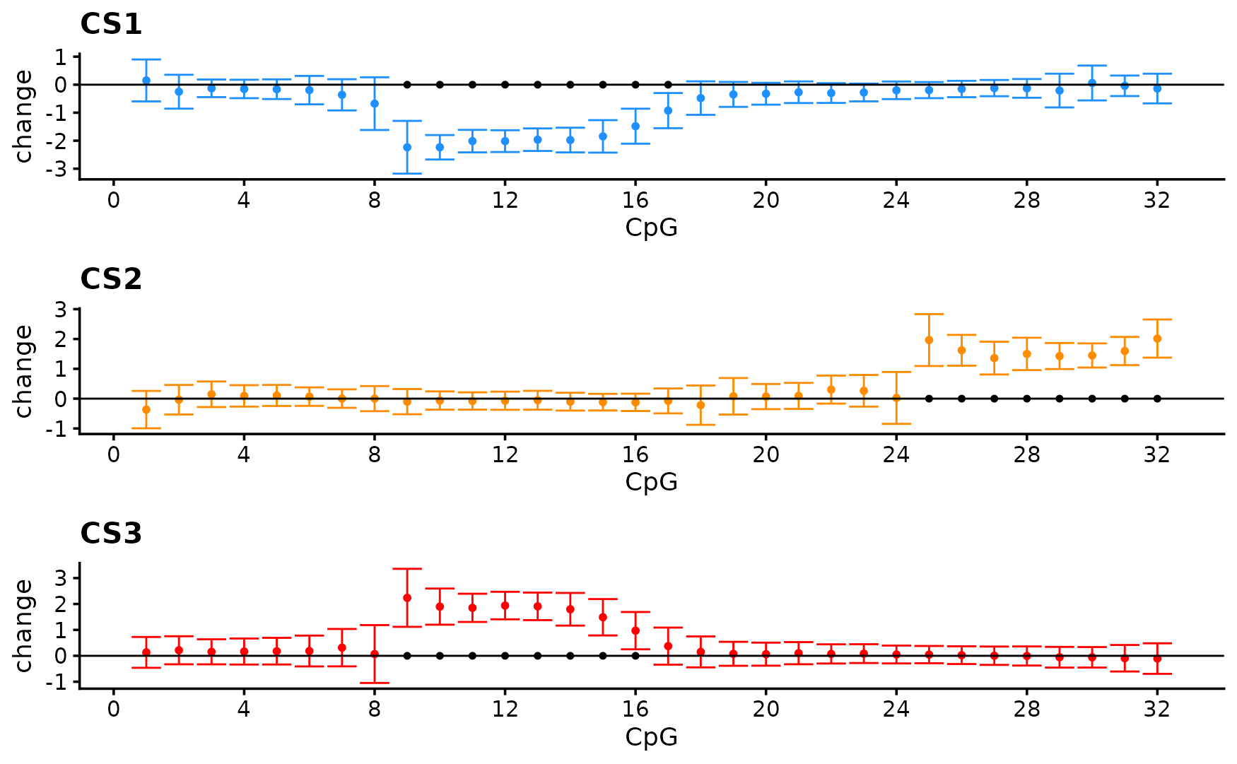
Running SuSiE on principal components (PCs)
Compute PCs
pca_res= prcomp(Y, center = TRUE, scale. = TRUE)Results on first PC
res_susie_PC1=susie(y=pca_res$x[,1],X)
res_susie_PC1$sets
# $cs
# $cs$L1
# [1] 9
#
# $cs$L2
# [1] 1
#
#
# $purity
#    min.abs.corr mean.abs.corr median.abs.corr
# L1            1             1               1
# L2            1             1               1
#
# $cs_index
# [1] 1 2
#
# $coverage
# [1] 1 1
#
# $requested_coverage
# [1] 0.95
We only capture the SNP that affect the lfetmost bump.
When running SusiE on the second PC we capture the SNP with the effect on the rightmost CpGs.
res_susie_PC2=susie(y=pca_res$x[,2],X)
res_susie_PC2$sets
# $cs
# $cs$L1
# [1] 3 4
#
#
# $purity
#    min.abs.corr mean.abs.corr median.abs.corr
# L1    0.9989364     0.9989364       0.9989364
#
# $cs_index
# [1] 1
#
# $coverage
# [1] 1
#
# $requested_coverage
# [1] 0.95
In this case we suspect that because most of the variation in the data is due to orthogonal effects and because principal components are orthogonal by construction then the first PC captures the effect of one of the SNP and has no information about the other SNP and vice versa.