Introduction to fSuSiE
William R.P. Denault
2026-05-13
Source:vignettes/fsusie_intro.Rmd
fsusie_intro.RmdOverview
fSuSiE implements a Bayesian variable selection method based on the “Functional Sum of Single Effects” (fSuSiE) model. The fSuSiE model extends the SuSiE model to functional traits. fSuSiE (and SuSiE) are particularly well suited to settings where some of the variables are strongly correlated and the true effects on the trait are very sparse. This is exactly the situation we face in genetic fine-mapping. The functional traits of interest are molecular measurements from sequencing assays (e.g., ChIP-seq, ATAC-seq), and DNA methylation. However, the methods are quite general and could be useful for other problems inside and outside genetics.
The fSuSiE model
fSuSiE fits the linear regression model {\bf Y} = {\bf X} {\bf B} + {\bf E},
where \bf Y is an N x T matrix containing the N trait observations at T locations; \bf X is the N x p matrix of single nucleotide polymorphisms (SNP) in the region to be fine-mapped; \bf B is a p x T matrix whose element b_{jt} is the effect of SNP j on the trait at location t; and \bf E is a matrix of error terms.
Analogous to regular fine-mapping, the matrix \bf B is expected to be row-wise sparse, that is, most of the rows of \bf B will be zero. (Non-zero rows correspond to SNPs that affect the trait.) The goal, in short, is to identify the non-zero rows of {\bf B}. To accomplish this task, we extend SuSiE to functional traits: we express {\bf B} as a sum of “single effects”, {\bf B} = \sum_{l=1}^L {B}^{(l)}, where each single-effect matrix {B}^{(l)} has only one non-zero row, corresponding to a single causal SNP. We have developed a fast procedure for fitting this model by (i) projecting the data in the wavelet space, then (ii) using a version of the iterative Bayesian stepwise selection (IBSS) algorithm adapted for fSuSiE.
fSuSiE also outputs Credible Sets (CSs). Each CS is defined so that it has a high probability of containing a variable with a non-zero effect while at the same time being as small as possible.
We illustrate these ideas in the examples below.
The example fine-mapping data set
library(susieR)
library(fsusieR)
#>
#> Attaching package: 'fsusieR'
#> The following object is masked from 'package:susieR':
#>
#>     get_objective
library(ggplot2)
library(cowplot)
We illustrate fSuSiE on a simulated molecular trait in which two of the candidate genetic variants (SNPs) affect the trait. The molecular trait spans a region of 120 locations.
First, we simulate the SNP effects (blue and green in the plot):
set.seed(1)
f1 <- simu_IBSS_per_level(7)$sim_func
f2 <- simu_IBSS_per_level(7)$sim_func
par(mar = c(2,2,2,2))
plot(f1,type = "l",col = "royalblue",lwd = 2)
abline(a = 0,b = 0,lty = "dotted")
lines(f2,type = "l",col = "limegreen",lwd = 2)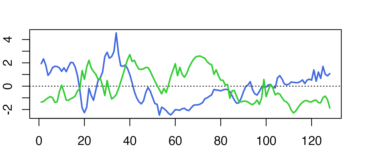
Notice that each of the SNPs increases or decreases at many locations, but in a mostly spatially smooth way.
Now we simulate the molecular trait. To do this, we use some genotype data included in susieR.
data(N3finemapping)
rsnr  <- 0.5
pos1  <- 25
pos2  <- 75
X     <- N3finemapping$X[,1:100]
n     <- nrow(X)
nloc  <- length(f1)
noise <- matrix(rnorm(n*nloc,sd = var(f1)/rsnr),n,nloc)
Y     <- tcrossprod(X[,pos1],f1) + tcrossprod(X[,pos2],f2) + noise
The end result is a fine-mapping data set containing the genotype data at 100 SNPs (stored as a 574 x 100 matrix {\bf X}) and the molecular trait data at 128 locations (stored as a 574 x 128 matrix {\bf Y}).
Note that the true causal SNPs are at SNP positions 25 and 75 (columns 25 and 75 in the X matrix).
Fitting the fSuSiE model
The main function in fsusieR for performing an fSuSiE analysis is the “susiF” function. It has many input arguments for customizing or fine-tuning the analysis, but at its simplest, only three inputs are needed: (1) the molecular trait matrix, \bf Y; (2) the genotype matrix, \bf X; and (3) a number specifying an upper bound on the number of single effects. Typically this number will be around 10, or perhaps a bit larger. Therefore, the call to susiF for this simulated data set is simply:
fit <- susiF(Y,X,L = 10)On most current computers, this call to susiF should not take more than a minute or two to run.
fSuSiE automatically selects the number of causal effects (here two). The effects detected are summarized in terms of credible sets (CSs). Each credible set contains the likely causal covariates for a given effect. You can access them simply as
fit$cs
#> [[1]]
#> [1] 75 83
#>
#> [[2]]
#> [1] 25
As you can see, the two CSs contain the correct causal SNPs.
cs1 <- fit$cs[[1]]
cs2 <- fit$cs[[2]]
fit$pip[cs1]
#> [1] 0.5 0.5
fit$pip[cs2]
#> [1] 1
cor(X[,cs1])
#>      [,1] [,2]
#> [1,]    1    1
#> [2,]    1    1
Visualization
You can also access the information directly in the output of susiF in the fitted_func part of the output. See below
plot_susiF_effect(fit)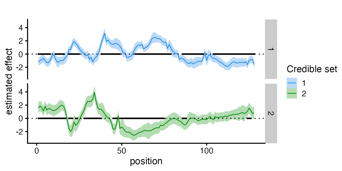
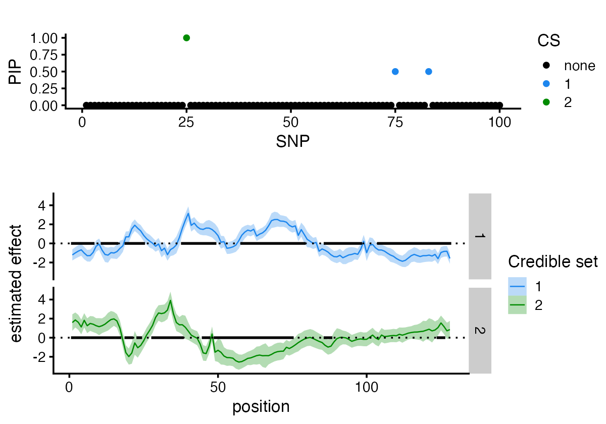
You can also access the posterior inclusion probabilities directly from the fitted object. Similarly, you can specify the plot_susiF function to display only the PiP plot.
plot_susiF_pip(fit)
Or use the “plot” method to quickly generate both plots.
Handling functions of any length and unevenly spaced data
Wavelets are primarily designed to analyze functions sampled on 2^J evenly spaced positions. However, this assumption can be limiting.
For handling functions of any length, we use the approach of Kovac and Silvermann (2005) which remaps the data on a grid of length 2^J.
Here are a couple of things to keep in mind:
If you don’t provide the sampling positions (e.g., base pair measurement) in the “pos” argument, susiF assumes that the columns of Y are evenly spaced. For molecular traits with known genomic positions (e.g., base-pair positions), we recommend providing the genomic positions in the “pos” argument.
susiF always returns the estimated effect on a 2^J grid.
To illustrate, consider the following example. The true function is defined on 2^9 = 512 positions, but we only observe the function in a random subset of those positions.
set.seed(2)
data(N3finemapping)
f1 <- simu_IBSS_per_level(9)$sim_func
f2 <- simu_IBSS_per_level(9)$sim_func
pos <- sort(sample(512,130))
par(mar = c(2,2,2,2))
plot(f2,type = "l",lwd = 1.25)
points(pos,f2[pos],col = "black",pch = 20,cex = 0.75)
abline(a = 0,b = 0,col = "black",lty = "dotted")
Let’s now generate the data matrix Y similar to above.
rsnr   <- 0.03
f1_obs <- f1[pos]
f2_obs <- f2[pos]
X      <- N3finemapping$X[,1:100]
n      <- nrow(X)
nloc   <- length(pos)
noise  <- matrix(rnorm(n*nloc,sd = var(f1)/rsnr),n,nloc)
Y      <- tcrossprod(X[,pos1],f1_obs) + tcrossprod(X[,pos2],f2_obs) + noise
The only change to the call to susiF is that we now also provide the sampling positions:
fit <- susiF(Y,X,L = 10,pos=pos)
#> Response matrix dimensions not equal to nx 2^J
#>  or unevenly spaced data
#>  interpolation procedure used
To visualize the estimated effects, again we can use the “plot_susiF_effect” function:
plot_susiF_effect(fit)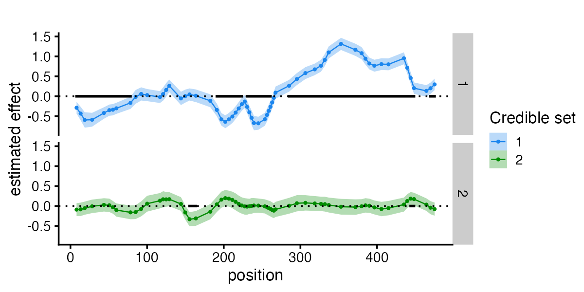
See how the estimated function recover the true underlying effect.
plot(fit$outing_grid, fit$fitted_func[[1]] , col="blue", type="l")
lines(fit$outing_grid, fit$cred_band[[1]][1,] , col="blue",lty=2)
lines(fit$outing_grid, fit$cred_band[[1]][2,] , col="blue",lty=2)

points(pos,f2[pos],col = "black",pch = 20,cex = 0.75)
lines(f2)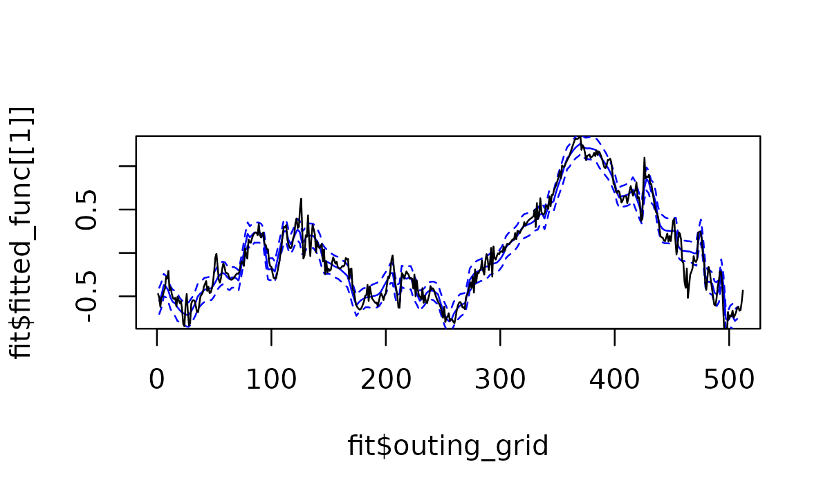
Prior on the effects
Note that fSuSiE has two different priors available: mixture_normal_per_scale and mixture_normal. The default value is mixture_normal_per_scale, which has slightly higher performance overall (power, estimation accuracy) than mixture_normal. However, mixture_normal is somewhat faster:
fit_mnps <- susiF(Y,X,L = 10,prior = "mixture_normal_per_scale",verbose = FALSE)
#> [1] "Fine mapping done, refining effect estimates using cylce spinning wavelet transform"
fit_mn <- susiF(Y,X,L = 10,prior = "mixture_normal",verbose = FALSE)
#> [1] "Fine mapping done, refining effect estimates using cylce spinning wavelet transform"
fit_mnps$runtime
#>    user  system elapsed
#> 524.043   1.162 295.375
fit_mn$runtime
#>    user  system elapsed
#> 591.131   0.813 194.234
Therefore, for larger data sets you may want to use the
prior = "mixture_normal" option.