Illustration of the limitations of SuSiE for molecular phenotype data

This vignette illustrates some of the limitations of SuSiE when analyzing molecular traits or traits/responses variables that are functions. We use a simple example where the effect of a SNP spans over multiple CpG. We start by fine-mapping the effect of the genotype on each CpG in a sequential fashion. Then, we show that SuSiE can output inconsistent results. We also look at mvSuSiE under different prior and residual-variance initializations. Finally we show that fSuSiE can handle this problem and output much more interpretable results.

library(fsusieR)
library(susieR)
library(ggplot2)
library(cowplot)

Simulation

Let’s simulate a simple effect of a SNP on a set of CpGs. The effect of the SNP is a cosine function that spans over 40 CpGs.

set.seed(1)
data(N3finemapping, package = "susieR")

X_full <- N3finemapping$X[seq_len(100), ]
T_m <- 128L

effect <- 1.2 * cos(seq_len(T_m) / T_m * 3 * pi)
effect[effect < 0] <- 0
effect[seq_len(40)] <- 0

true_pos <- 700L
y <- matrix(0, nrow = 100L, ncol = T_m)
for (i in seq_len(100L)) {
  y[i, ] <- X_full[i, true_pos] * effect + rnorm(T_m)
}

col_var <- apply(X_full, 2, var)
keep <- which(col_var > 0)
X <- X_full[, keep]
true_pos_filt <- which(keep == true_pos)
affected_pos <- which(effect > 0)

plot(effect, pch = 19, xlab = "CpG", ylab = "effect")

We simulate 100 observations of the effect of the SNP on the CpG. The original causal SNP index is 700. The genotype matrix has a few constant columns in these 100 samples, so these columns are removed before fitting the models. This matters for interpreting SNP indices: the original causal SNP 700 is index 691 in the filtered design matrix.

data.frame(
  N = nrow(X),
  J = ncol(X),
  T = ncol(y),
  true_snp_original = true_pos,
  true_snp_filtered = true_pos_filt,
  affected_start = min(affected_pos),
  affected_end = max(affected_pos),
  affected_positions = length(affected_pos)
)
#>     N   J   T true_snp_original true_snp_filtered affected_start affected_end
#> 1 100 991 128               700               691             65          106
#>   affected_positions
#> 1                 42

Method 1: Per-CpG SuSiE

Once the data is simulated, we can run SuSiE on each CpG. For the sake of simplicity, we only run SuSiE with L = 1 as we are aware that there is only one effect in this simulation. Also for simplicity, we assume that the association analysis has been performed with 100% accuracy—that is, we know exactly which CpGs are the affected CpGs, and therefore we can ignore the others.

susie_est <- vector("list", length(affected_pos))
for (k in seq_along(affected_pos)) {
  susie_est[[k]] <- susie(X, y[, affected_pos[k]], L = 1L)$sets
}
n_cs_per_pos <- vapply(susie_est, function(s) length(s$cs), integer(1L))

knitr::kable(
  data.frame(
    n_credible_sets = as.integer(names(table(n_cs_per_pos))),
    n_positions = as.integer(table(n_cs_per_pos))
  )
)

n_credible_sets	n_positions
0	36
1	6

One issue is that SuSiE fails to detect a causal SNP at most of the affected CpGs:

df_effect <- data.frame(position = seq_along(effect), effect = effect)

plot_effect_position <- function(pos) {
  ggplot(df_effect, aes(x = position, y = effect)) +
    geom_point(color = "grey55", size = 1.2) +
    geom_hline(yintercept = 0, linetype = "dotted", color = "grey50") +
    geom_point(data = df_effect[pos, , drop = FALSE],
               color = "firebrick", size = 2.4) +
    labs(x = "CpG position", y = "true effect",
         title = paste("Position", pos)) +
    theme_classic()
}

plot_susie_position <- function(pos) {
  fit <- susie(X, y[, pos], L = 1L)
  df_pip <- data.frame(snp = keep, pip = fit$pip)
  p <- ggplot(df_pip, aes(x = snp, y = pip)) +
    geom_point(color = "grey55", size = 0.8) +
    geom_vline(xintercept = true_pos, linetype = "dashed",
               color = "firebrick", alpha = 0.7) +
    geom_point(data = df_pip[df_pip$snp == true_pos, , drop = FALSE],
               color = "firebrick", shape = 21, size = 2.3, stroke = 1.1) +
    coord_cartesian(ylim = c(0, 1)) +
    labs(x = "SNP original index", y = "PIP",
         title = paste("SuSiE PIP at position", pos)) +
    theme_classic()
  cs <- fit$sets$cs$L1
  if (!is.null(cs)) {
    p <- p + geom_point(data = df_pip[cs, , drop = FALSE],
                        color = "dodgerblue", size = 1.8)
  }
  p
}

plot_grid(
  plot_effect_position(88L), plot_effect_position(91L),
  plot_susie_position(88L), plot_susie_position(91L),
  nrow = 2L, ncol = 2L
)

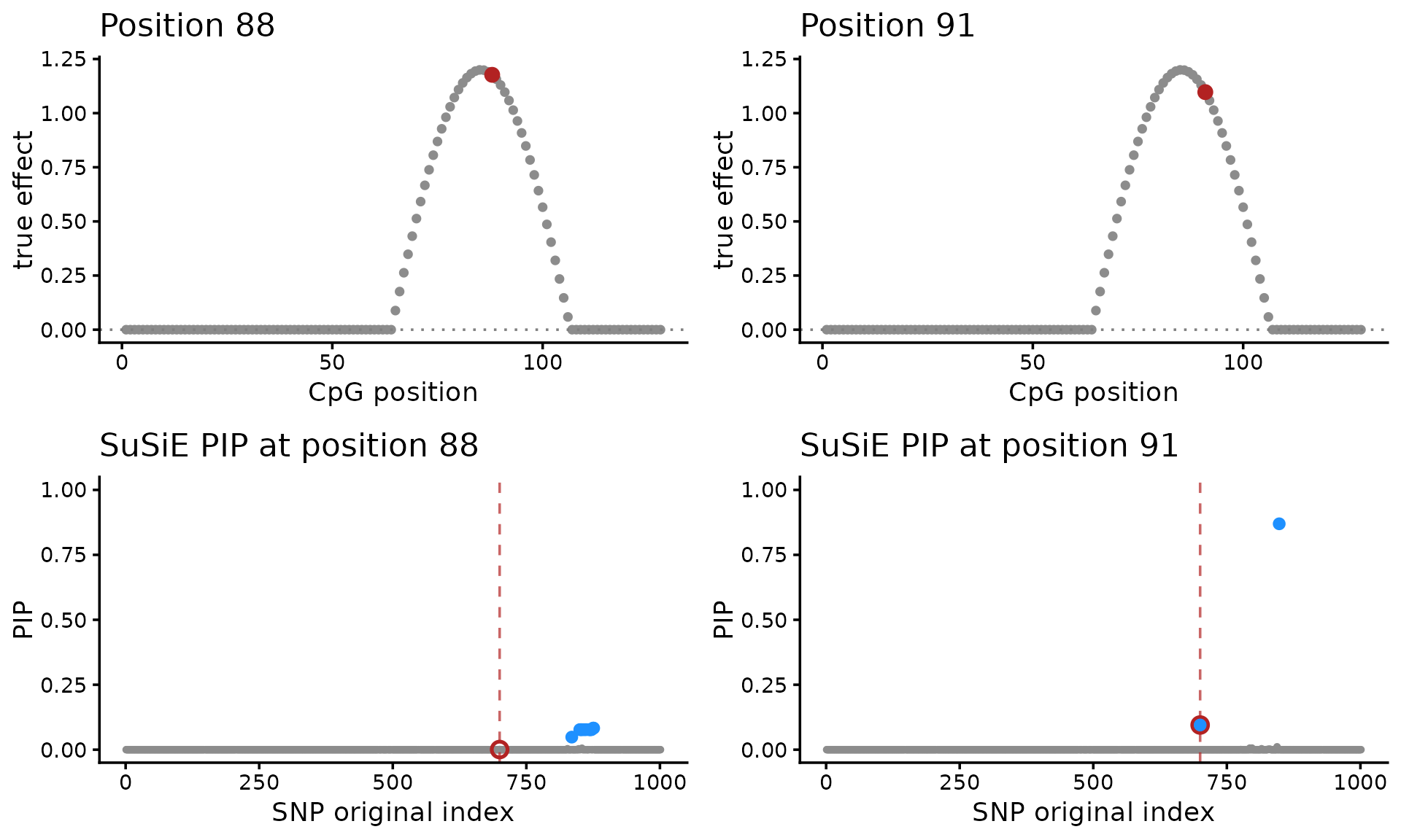
A second issue is that the SuSiE produces multiple fine-mapping signals (and therefore multiple sets of CSs), so it is unclear how to reason about uncertainty in the causal SNP(s). For example, compare the SuSiE results for CpGs 88 and 91. At CpG 88, the credible set misses the true SNP. At CpG 91, the true SNP is present, but it is not the lead variant.

Method 2: mvSuSiE

mvSuSiE treats Y as a multivariate response. Its behavior depends strongly on the prior and residual-variance initialization. The “oracle” residual variance is the identity matrix used to simulate the data, and the “oracle” prior is the outer product of the true effect curve with itself. The PIP-zero failure mode of the default mvSuSiE on this simulation is the subject of mvsusieR issue 61.

library(mvsusieR)

U_true <- outer(effect, effect)
prior_true <- create_mixture_prior(
  mixture_prior = list(matrices = list(U_true), weights = 1)
)
prior_canon <- create_mixture_prior(R = T_m)
V_true <- diag(T_m)

run_mvsusie <- function(...) {
  suppressWarnings(mvsusie(..., verbose = FALSE))
}

get_mvsusie_curve <- function(fit) {
  as.numeric(coef(fit)[true_pos_filt + 1L, ])
}

curve_cor <- function(curve) {
  if (sd(curve) == 0) {
    NA_real_
  } else {
    cor(curve, effect)
  }
}

summarize_mvsusie <- function(fit, label, prior, residual, init) {
  curve <- get_mvsusie_curve(fit)
  data.frame(
    test = label,
    prior = prior,
    residual_variance = residual,
    initialization = init,
    pip_at_true_snp = fit$pip[true_pos_filt],
    max_pip = max(fit$pip),
    lead_snp_original = keep[which.max(fit$pip)],
    n_cs = length(fit$sets$cs),
    effect_cor = curve_cor(curve),
    max_abs_effect = max(abs(curve)),
    converged = isTRUE(fit$converged)
  )
}

fit_mv1 <- run_mvsusie(
  X, y, L = 1L,
  prior_variance = prior_true,
  residual_variance = V_true,
  estimate_residual_variance = FALSE,
  estimate_prior_variance = TRUE,
  max_iter = 100L
)

fit_mv2 <- run_mvsusie(
  X, y, L = 1L,
  prior_variance = prior_true,
  residual_variance = V_true,
  estimate_residual_variance = TRUE,
  estimate_prior_variance = TRUE,
  max_iter = 100L
)

fit_mv3 <- run_mvsusie(
  X, y, L = 1L,
  prior_variance = prior_canon,
  residual_variance = V_true,
  estimate_residual_variance = FALSE,
  estimate_prior_variance = TRUE,
  max_iter = 100L
)

fit_mv4 <- run_mvsusie(
  X, y, L = 1L,
  prior_variance = prior_true,
  estimate_residual_variance = TRUE,
  estimate_prior_variance = TRUE,
  max_iter = 100L
)

fit_mv5 <- run_mvsusie(
  X, y, L = 1L,
  prior_variance = prior_true,
  estimate_residual_variance = FALSE,
  estimate_prior_variance = TRUE,
  max_iter = 100L
)

fit_mv6 <- run_mvsusie(
  X, y, L = 1L,
  prior_variance = prior_canon,
  estimate_residual_variance = TRUE,
  estimate_prior_variance = TRUE,
  max_iter = 100L
)

fit_mv7 <- run_mvsusie(
  X, y, L = 1L,
  prior_variance = prior_canon,
  estimate_residual_variance = FALSE,
  estimate_prior_variance = TRUE,
  max_iter = 100L
)

mv_table <- rbind(
  summarize_mvsusie(fit_mv1, "1", "oracle", "oracle fixed",
                    "oracle residual"),
  summarize_mvsusie(fit_mv2, "2", "oracle", "estimated",
                    "oracle residual"),
  summarize_mvsusie(fit_mv3, "3", "canonical", "oracle fixed",
                    "oracle residual"),
  summarize_mvsusie(fit_mv4, "4", "oracle", "estimated", "default"),
  summarize_mvsusie(fit_mv5, "5", "oracle", "default fixed", "default"),
  summarize_mvsusie(fit_mv6, "6", "canonical", "estimated", "default"),
  summarize_mvsusie(fit_mv7, "7", "canonical", "default fixed", "default")
)

The tuned configuration recovers the effect shape closely. The default configuration’s recovered curve is essentially flat at zero: with no truth-informed residual-variance initialization, the PIPs collapse and the fitted effect carries no information.

curve_mv_oracle <- get_mvsusie_curve(fit_mv1)
curve_mv_default <- get_mvsusie_curve(fit_mv6)

yrng <- range(c(effect, curve_mv_oracle, curve_mv_default))
plot_mv_curve <- function(curve, main) {
  plot(effect, pch = 20L, col = "grey30", cex = 0.7, ylim = yrng,
       xlab = "position", ylab = "effect", main = main)
  abline(h = 0, lty = 3, col = "grey50")
  lines(curve, col = "firebrick", lwd = 2)
}

par(mfrow = c(1L, 2L), mar = c(4, 4, 2.5, 1))
plot_mv_curve(curve_mv_oracle,
              "mvSuSiE, oracle initialized")
plot_mv_curve(curve_mv_default,
              "mvSuSiE, default")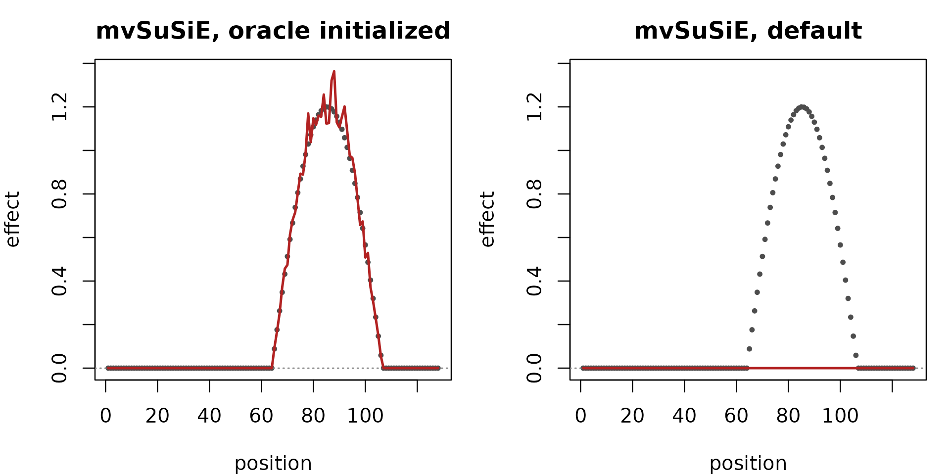

par(mfrow = c(1L, 1L))

The table repeats the same simulation under several configurations:

knitr::kable(mv_table, digits = 4)

	test	prior	residual_variance	initialization	pip_at_true_snp	max_pip	lead_snp_original	n_cs	effect_cor	max_abs_effect	converged
var691	1	oracle	oracle fixed	oracle residual	1	1	700	1	0.9972	1.3637	TRUE
var6911	2	oracle	estimated	oracle residual	1	1	700	1	0.9972	1.3636	FALSE
var6912	3	canonical	oracle fixed	oracle residual	1	1	700	1	0.8909	1.1128	TRUE
var6913	4	oracle	estimated	default	0	0	1	0	NA	0.0000	TRUE
var6914	5	oracle	default fixed	default	0	0	1	0	NA	0.0000	TRUE
var6915	6	canonical	estimated	default	0	0	1	0	NA	0.0000	TRUE
var6916	7	canonical	default fixed	default	0	0	1	0	NA	0.0000	TRUE

The first three configurations recover the true SNP. All three use the correct residual-variance initialization. The default initializations fail: the PIPs collapse to zero and no credible set is returned.

Method 3: fSuSiE

Now compare to an analysis of these data using fSuSiE, which involves a single call to the “susiF” function. Here we use trend-filtering post-processing.

fit_f <- susiF(y, X, L = 1L, post_processing = "TI", verbose = FALSE)

fit_f$cs
fit_f$pip[true_pos_filt]
#> [1] "Fine mapping done, refining effect estimates using cylce spinning wavelet transform"
#> [[1]]
#> [1] 691
#> 
#> [1] 1

Notice that fSuSiE returned a single CS containing 1 SNP, which is the true causal SNP.

df_f_pip <- data.frame(snp = keep, pip = fit_f$pip)
P_pip <- ggplot(df_f_pip, aes(x = snp, y = pip)) +
  geom_point(color = "grey55", size = 0.8) +
  geom_vline(xintercept = true_pos, linetype = "dashed",
             color = "firebrick", alpha = 0.7) +
  geom_point(data = df_f_pip[df_f_pip$snp == true_pos, , drop = FALSE],
             color = "firebrick", size = 2.3) +
  coord_cartesian(ylim = c(0, 1)) +
  labs(x = "SNP original index", y = "PIP", title = "fSuSiE PIPs") +
  theme_classic()

df_f_curve <- data.frame(
  position = seq_along(fit_f$fitted_func[[1]]),
  estimate = fit_f$fitted_func[[1]],
  upper = fit_f$cred_band[[1]][1, ],
  lower = fit_f$cred_band[[1]][2, ],
  truth = effect
)

P_effect <- ggplot(df_f_curve, aes(x = position)) +
  geom_ribbon(aes(ymin = lower, ymax = upper), fill = "skyblue",
              alpha = 0.45) +
  geom_point(aes(y = truth), color = "grey30", size = 1.1) +
  geom_line(aes(y = estimate), color = "firebrick", linewidth = 1) +
  geom_hline(yintercept = 0, linetype = "dotted", color = "grey50") +
  labs(x = "CpG position", y = "effect",
       title = "fSuSiE recovered effect curve") +
  theme_classic()

plot_grid(P_pip, P_effect, nrow = 1L, rel_widths = c(1, 1.25))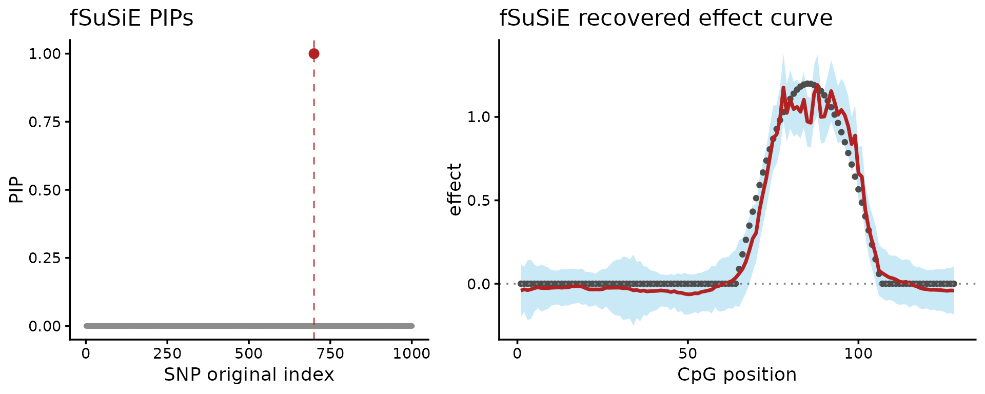

These plots show two other results: on the left-hand side, the fine-mapping signal (PIPs); on the right-hand side, the estimated effect on the methylation levels (red = posterior mean, light blue = credible bands). Together, these are the outputs needed to reason about both the causal SNP and the shape of its effect across CpGs.

William R.P. Denault and Gao Wang

2024-03-07

Simulation

Method 1: Per-CpG SuSiE

Method 2: mvSuSiE

Method 3: fSuSiE