Predict loadings based on previously fit Poisson NMF,
or predict topic proportions based on previously fit multinomial
topic model. This can be thought of as projecting data points onto
a previously estimated set of factors fit$F.
Arguments
- object
An object of class “poisson_nmf_fit” or “multinom_topic_model_fit”.
- newdata
An optional counts matrix. If omitted, the loadings estimated in the original data are returned.
- numiter
The number of updates to perform.
- ...
Additional arguments passed to
fit_poisson_nmf.
Value
A loadings matrix with one row for each data point and one
column for each topic or factor. For
predict.multinom_topic_model_fit, the output can also be
interpreted as a matrix of estimated topic proportions, in which
L[i,j] is the proportional contribution of topic j to data
point i.
See also
Examples
# \donttest{
# Simulate a 175 x 1,200 counts matrix.
set.seed(1)
dat <- simulate_count_data(175,1200,k = 3)
# Split the data into training and test sets.
train <- dat$X[1:100,]
test <- dat$X[101:175,]
# Fit a Poisson non-negative matrix factorization using the
# training data.
fit <- init_poisson_nmf(train,F = dat$F,init.method = "random")
fit <- fit_poisson_nmf(train,fit0 = fit)
#> Fitting rank-3 Poisson NMF to 100 x 1200 dense matrix.
#> Running at most 100 SCD updates, without extrapolation (fastTopics 0.7-38).
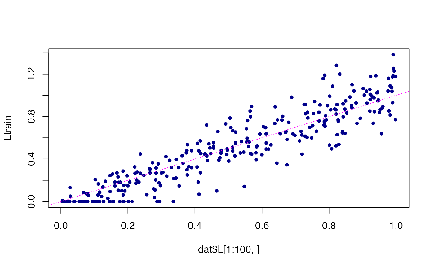
# Compare the estimated loadings in the training data against the
# loadings used to simulate these data.
Ltrain <- predict(fit)
plot(dat$L[1:100,],Ltrain,pch = 20,col = "darkblue")
abline(a = 0,b = 1,col = "magenta",lty = "dotted",
xlab = "true",ylab = "estimated")
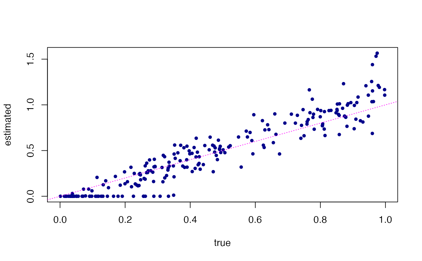
 # Next, predict loadings in unseen (test) data points, and compare
# these predictions against the loadings that were used to simulate
# the test data.
Ltest <- predict(fit,test)
#> Fitting rank-3 Poisson NMF to 75 x 1200 dense matrix.
#> Running at most 20 SCD updates, without extrapolation (fastTopics 0.7-38).
plot(dat$L[101:175,],Ltest,pch = 20,col = "darkblue",
xlab = "true",ylab = "estimated")
abline(a = 0,b = 1,col = "magenta",lty = "dotted")
# Next, predict loadings in unseen (test) data points, and compare
# these predictions against the loadings that were used to simulate
# the test data.
Ltest <- predict(fit,test)
#> Fitting rank-3 Poisson NMF to 75 x 1200 dense matrix.
#> Running at most 20 SCD updates, without extrapolation (fastTopics 0.7-38).
plot(dat$L[101:175,],Ltest,pch = 20,col = "darkblue",
xlab = "true",ylab = "estimated")
abline(a = 0,b = 1,col = "magenta",lty = "dotted")
 # Simulate a 175 x 1,200 counts matrix.
set.seed(1)
dat <- simulate_multinom_gene_data(175,1200,k = 3)
# Split the data into training and test sets.
train <- dat$X[1:100,]
test <- dat$X[101:175,]
# Fit a topic model using the training data.
fit <- init_poisson_nmf(train,F = dat$F,init.method = "random")
fit <- fit_poisson_nmf(train,fit0 = fit)
#> Fitting rank-3 Poisson NMF to 100 x 1200 dense matrix.
#> Running at most 100 SCD updates, without extrapolation (fastTopics 0.7-38).
fit <- poisson2multinom(fit)
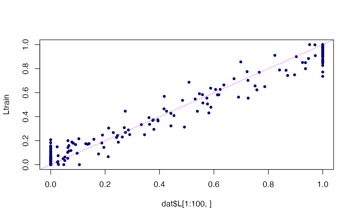
# Compare the estimated topic proportions in the training data against
# the topic proportions used to simulate these data.
Ltrain <- predict(fit)
plot(dat$L[1:100,],Ltrain,pch = 20,col = "darkblue")
abline(a = 0,b = 1,col = "magenta",lty = "dotted",
xlab = "true",ylab = "estimated")
# Simulate a 175 x 1,200 counts matrix.
set.seed(1)
dat <- simulate_multinom_gene_data(175,1200,k = 3)
# Split the data into training and test sets.
train <- dat$X[1:100,]
test <- dat$X[101:175,]
# Fit a topic model using the training data.
fit <- init_poisson_nmf(train,F = dat$F,init.method = "random")
fit <- fit_poisson_nmf(train,fit0 = fit)
#> Fitting rank-3 Poisson NMF to 100 x 1200 dense matrix.
#> Running at most 100 SCD updates, without extrapolation (fastTopics 0.7-38).
fit <- poisson2multinom(fit)
# Compare the estimated topic proportions in the training data against
# the topic proportions used to simulate these data.
Ltrain <- predict(fit)
plot(dat$L[1:100,],Ltrain,pch = 20,col = "darkblue")
abline(a = 0,b = 1,col = "magenta",lty = "dotted",
xlab = "true",ylab = "estimated")
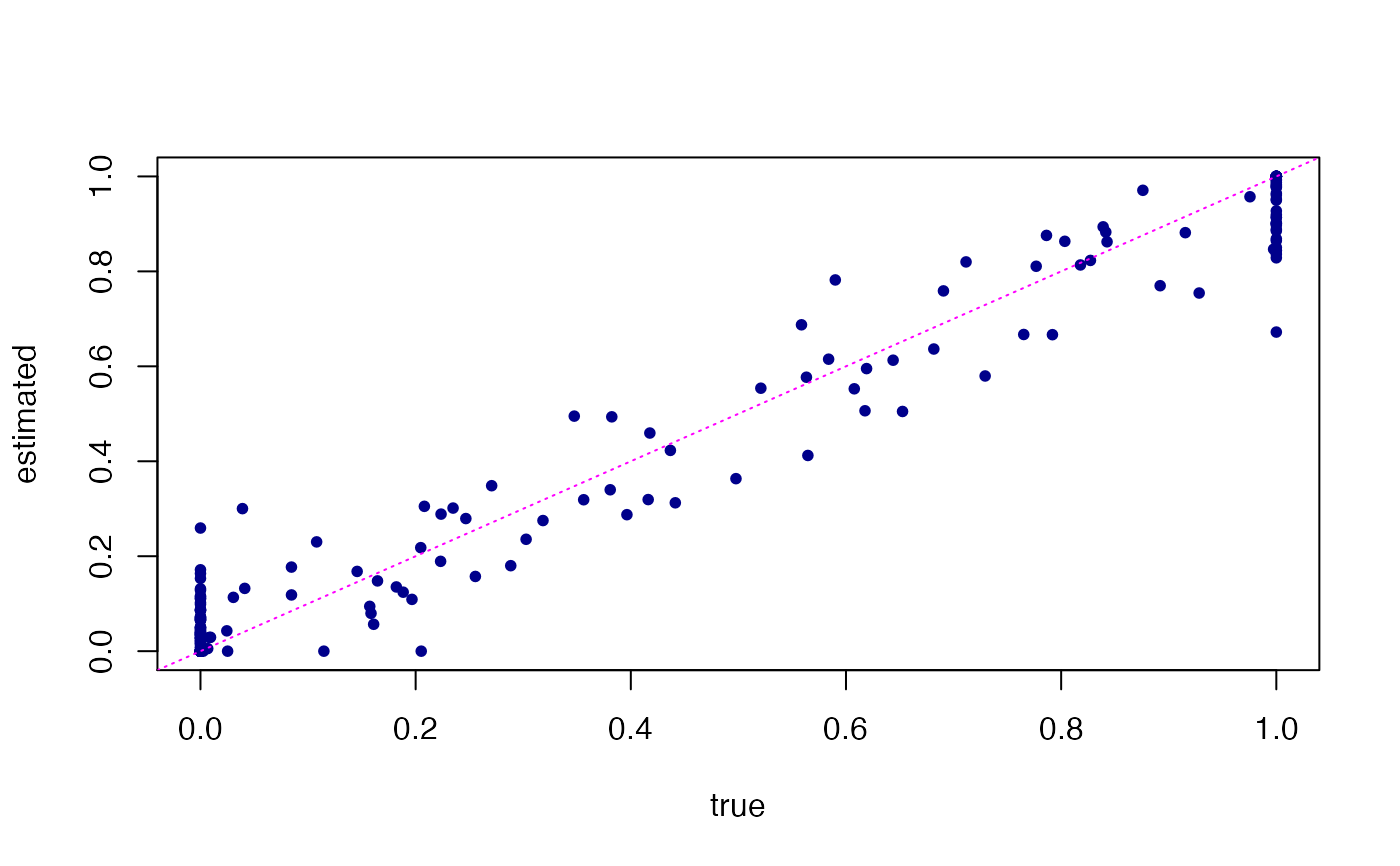
 # Next, predict loadings in unseen (test) data points, and compare
# these predictions against the loadings that were used to simulate
# the test data.
Ltest <- predict(fit,test)
#> Fitting rank-3 Poisson NMF to 75 x 1200 dense matrix.
#> Running at most 20 SCD updates, without extrapolation (fastTopics 0.7-38).
plot(dat$L[101:175,],Ltest,pch = 20,col = "darkblue",
xlab = "true",ylab = "estimated")
abline(a = 0,b = 1,col = "magenta",lty = "dotted")
# Next, predict loadings in unseen (test) data points, and compare
# these predictions against the loadings that were used to simulate
# the test data.
Ltest <- predict(fit,test)
#> Fitting rank-3 Poisson NMF to 75 x 1200 dense matrix.
#> Running at most 20 SCD updates, without extrapolation (fastTopics 0.7-38).
plot(dat$L[101:175,],Ltest,pch = 20,col = "darkblue",
xlab = "true",ylab = "estimated")
abline(a = 0,b = 1,col = "magenta",lty = "dotted")
 # }
# }