Fit Non-negative Matrix Factorization to Count Data

Approximate the input matrix X by the non-negative matrix factorization tcrossprod(L,F), in which the quality of the approximation is measured by a “divergence” criterion; equivalently, optimize the likelihood under a Poisson model of the count data, X, in which the Poisson rates are given by tcrossprod(L,F). Function fit_poisson_nmf runs a specified number of coordinate-wise updates to fit the L and F matrices.

fit_poisson_nmf(
  X,
  k,
  fit0,
  numiter = 100,
  update.factors = seq(1, ncol(X)),
  update.loadings = seq(1, nrow(X)),
  method = c("scd", "em", "mu", "ccd"),
  init.method = c("topicscore", "random"),
  control = list(),
  verbose = c("progressbar", "detailed", "none")
)

fit_poisson_nmf_control_default()

init_poisson_nmf(
  X,
  F,
  L,
  k,
  init.method = c("topicscore", "random"),
  beta = 0.5,
  betamax = 0.99,
  control = list(),
  verbose = c("detailed", "none")
)

init_poisson_nmf_from_clustering(X, clusters, ...)

Arguments

X

The n x m matrix of counts; all entries of X should be non-negative. It can be a sparse matrix (class "dgCMatrix") or dense matrix (class "matrix"), with some exceptions (see ‘Details’).

k

An integer 2 or greater giving the matrix rank. This argument should only be specified if the initial fit (fit0 or F, L) is not provided.

fit0

The initial model fit. It should be an object of class “poisson_nmf_fit”, such as an output from init_poisson_nmf, or from a previous call to fit_poisson_nmf.

numiter

The maximum number of updates of the factors and loadings to perform.

update.factors

A numeric vector specifying which factors (rows of F) to update. By default, all factors are updated. Note that the rows that are not updated may still change by rescaling. When NULL, all factors are fixed. This option is only implemented for method = "em" and method = "scd". If another method is selected, the default setting of update.factors must be used.

update.loadings

A numeric vector specifying which loadings (rows of L) to update. By default, all loadings are updated. Note that the rows that are not updated may still change by rescaling. When NULL, all loadings are fixed. This option is only implemented for method = "em" and method = "scd". If another method is selected, the default setting of update.loadings must be used.

method

The method to use for updating the factors and loadings. Four methods are implemented: multiplicative updates, method = "mu"; expectation maximization (EM), method = "em"; sequential co-ordinate descent (SCD), method = "scd"; and cyclic co-ordinate descent (CCD), method = "ccd". See ‘Details’ for a detailed description of these methods.

init.method

The method used to initialize the factors and loadings. When init.method = "random", the factors and loadings are initialized uniformly at random; when init.method = "topicscore", the factors are initialized using the (very fast) Topic SCORE algorithm (Ke & Wang, 2017), and the loadings are initialized by running a small number of SCD updates. This input argument is ignored if initial estimates of the factors and loadings are already provided via input fit0, or inputs F and L.

control

A list of parameters controlling the behaviour of the optimization algorithm (and the Topic SCORE algorithm if it is used to initialize the model parameters). See ‘Details’.

verbose

When verbose = "detailed", information about the algorithm's progress is printed to the console at each iteration; when verbose = "progressbar", a progress bar is shown; and when verbose = "none", no progress information is printed. See the description of the “progress” return value for an explanation of verbose = "detailed" console output. (Note that some columns of the “progress” data frame are not shown in the console output.)

F

An optional argument giving is the initial estimate of the factors (also known as “basis vectors”). It should be an m x k matrix, where m is the number of columns in the counts matrix X, and k > 1 is the rank of the matrix factorization (equivalently, the number of “topics”). All entries of F should be non-negative. When F and L are not provided, input argument k should be specified instead.

L

An optional argument giving the initial estimate of the loadings (also known as “activations”). It should be an n x k matrix, where n is the number of rows in the counts matrix X, and k > 1 is the rank of the matrix factorization (equivalently, the number of “topics”). All entries of L should be non-negative. When F and L are not provided, input argument k should be specified instead.

beta

Initial setting of the extrapolation parameter. This is \(beta\) in Algorithm 3 of Ang & Gillis (2019).

betamax

Initial setting for the upper bound on the extrapolation parameter. This is \(\bar{\gamma}\) in Algorithm 3 of Ang & Gillis (2019).

clusters

A factor specifying a grouping, or clustering, of the rows of X.

...

Additional arguments passed to init_poisson_nmf.

Value

init_poisson_nmf and fit_poisson_nmf both return an object capturing the optimization algorithm state (for init_poisson_nmf, this is the initial state). It is a list with the following elements:

F

A matrix containing the current best estimates of the factors.

L

A matrix containing the current best estimates of the loadings.

Fn

A matrix containing the non-extrapolated factor estimates. If extrapolation is not used, Fn and F will be the same.

Ln

A matrix containing the non-extrapolated estimates of the loadings. If extrapolation is not used, Ln and L will be the same.

Fy

A matrix containing the extrapolated factor estimates. If the extrapolation scheme is not used, Fy and F will be the same.

Ly

A matrix containing the extrapolated estimates of the loadings. If extrapolation is not used, Ly and L will be the same.

loss

Value of the objective (“loss”) function computed at the current best estimates of the factors and loadings.

loss.fnly

Value of the objective (“loss”) function computed at the extrapolated solution for the loadings (Ly) and the non-extrapolated solution for the factors (Fn). This is used internally to implement the extrapolated updates.

iter

The number of the most recently completed iteration.

beta

The extrapolation parameter, \(beta\) in Algorithm 3 of Ang & Gillis (2019).

betamax

Upper bound on the extrapolation parameter. This is \(\bar{\gamma}\) in Algorithm 3 of Ang & Gillis (2019).

beta0

The setting of the extrapolation parameter at the last iteration that improved the solution.

progress

A data frame containing detailed information about the algorithm's progress. The data frame should have at most numiter rows. The columns of the data frame are: “iter”, the iteration number; “loglik”, the Poisson NMF log-likelihood at the current best factor and loading estimates; “loglik.multinom”, the multinomial topic model log-likelihood at the current best factor and loading estimates; “dev”, the deviance at the current best factor and loading estimates; “res”, the maximum residual of the Karush-Kuhn-Tucker (KKT) first-order optimality conditions at the current best factor and loading estimates; “delta.f”, the largest change in the factors matrix; “delta.l”, the largest change in the loadings matrix; “nonzeros.f”, the proportion of entries in the factors matrix that are nonzero; “nonzeros.l”, the proportion of entries in the loadings matrix that are nonzero; “extrapolate”, which is 1 if extrapolation is used, otherwise it is 0; “beta”, the setting of the extrapolation parameter; “betamax”, the setting of the extrapolation parameter upper bound; and “timing”, the elapsed time in seconds (recorded using proc.time).

Details

In Poisson non-negative matrix factorization (Lee & Seung, 2001), counts \(x_{ij}\) in the \(n \times m\) matrix, \(X\), are modeled by the Poisson distribution: $$x_{ij} \sim \mathrm{Poisson}(\lambda_{ij}).$$ Each Poisson rate, \(\lambda_{ij}\), is a linear combination of parameters \(f_{jk} \geq 0, l_{ik} \geq 0\) to be fitted to the data: $$\lambda_{ij} = \sum_{k=1}^K l_{ik} f_{jk},$$ in which \(K\) is a user-specified tuning parameter specifying the rank of the matrix factorization. Function fit_poisson_nmf computes maximum-likelihood estimates (MLEs) of the parameters. For additional mathematical background, and an explanation of how Poisson NMF is connected to topic modeling, see the vignette: vignette(topic = "relationship",package = "fastTopics").

Using this function requires some care; only minimal argument checking is performed, and error messages may not be helpful.

The EM and multiplicative updates are simple and fast, but can be slow to converge to a stationary point. When control$numiter = 1, the EM and multiplicative updates are mathematically equivalent to the multiplicative updates, and therefore share the same convergence properties. However, the implementation of the EM updates is quite different; in particular, the EM updates are more suitable for sparse counts matrices. The implementation of the multiplicative updates is adapted from the MATLAB code by Daichi Kitamura http://d-kitamura.net.

Since the multiplicative updates are implemented using standard matrix operations, the speed is heavily dependent on the BLAS/LAPACK numerical libraries used. In particular, using optimized implementations such as OpenBLAS or Intel MKL can result in much improved performance of the multiplcative updates.

The cyclic co-ordinate descent (CCD) and sequential co-ordinate descent (SCD) updates adopt the same optimization strategy, but differ in the implementation details. In practice, we have found that the CCD and SCD updates arrive at the same solution when initialized “sufficiently close” to a stationary point. The CCD implementation is adapted from the C++ code developed by Cho-Jui Hsieh and Inderjit Dhillon, which is available for download at https://www.cs.utexas.edu/~cjhsieh/nmf/. The SCD implementation is based on version 0.4-3 of the ‘NNLM’ package.

An additional re-scaling step is performed after each update to promote numerical stability.

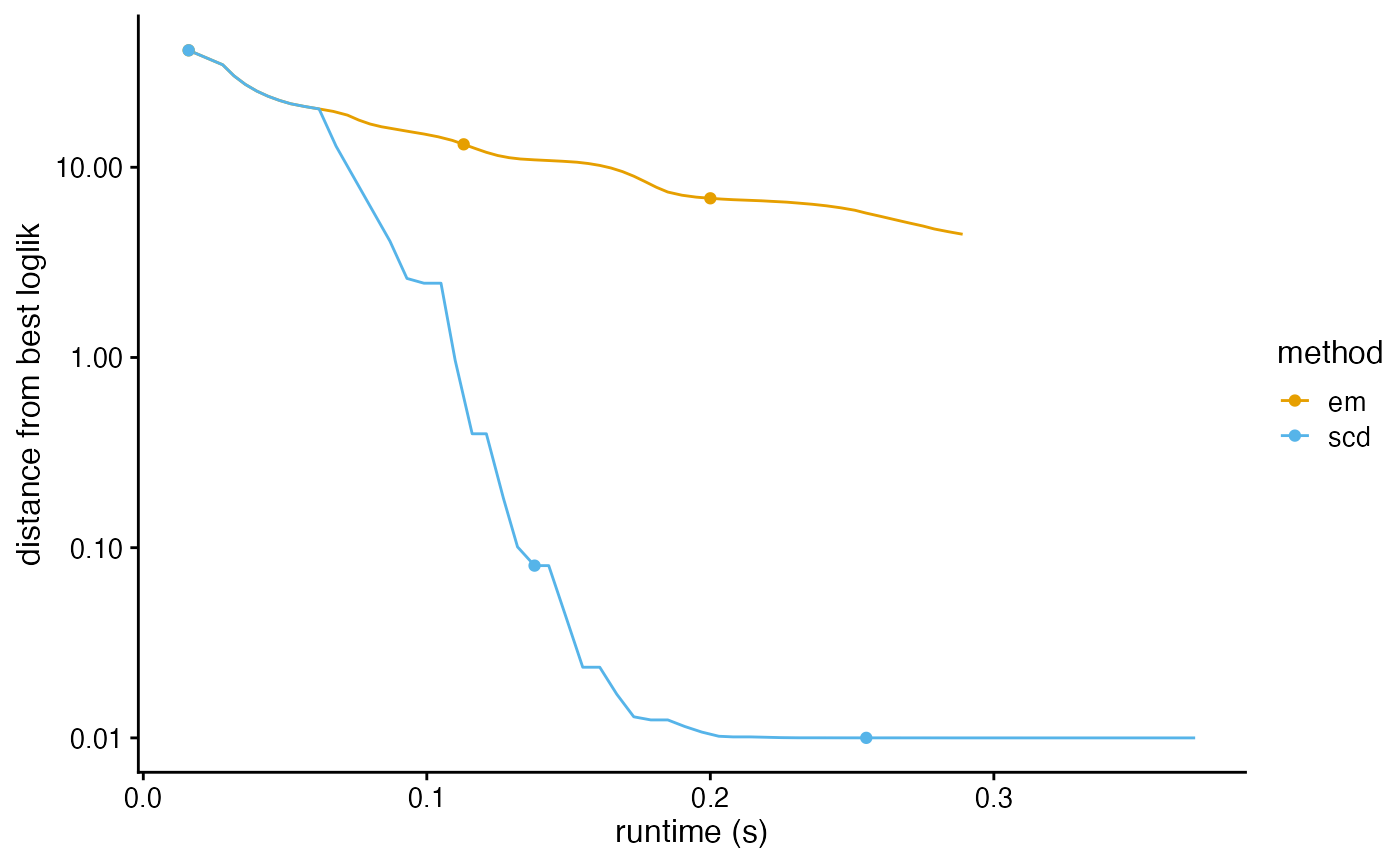
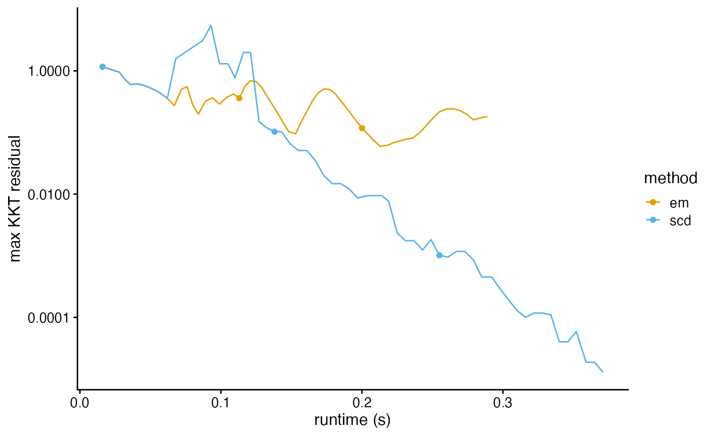
We use three measures of progress for the model fitting: (1) improvement in the log-likelihood (or deviance), (2) change in the model parameters, and (3) the residuals of the Karush-Kuhn-Tucker (KKT) first-order conditions. As the iterates approach a stationary point of the loss function, the change in the model parameters should be small, and the residuals of the KKT system should vanish. Use plot_progress to plot the improvement in the solution over time.

See fit_topic_model for additional guidance on model fitting, particularly for large or complex data sets.

The control argument is a list in which any of the following named components will override the default optimization algorithm settings (as they are defined by fit_poisson_nmf_control_default):

numiter

Number of “inner loop” iterations to run when performing and update of the factors or loadings. This must be set to 1 for method = "mu" and method = "ccd".

nc

Number of RcppParallel threads to use for the updates. When nc is NA, the number of threads is determined by calling defaultNumThreads. This setting is ignored for the multiplicative upates (method = "mu").

nc.blas

Number of threads used in the numerical linear algebra library (e.g., OpenBLAS), if available. For best performance, we recommend setting this to 1 (i.e., no multithreading).

min.delta.loglik

Stop performing updates if the difference in the Poisson NMF log-likelihood between two successive updates is less than min.delta.loglik. This should not be kept at zero when control$extrapolate = TRUE because the extrapolated updates are expected to occasionally keep the likelihood unchanged. Ignored if min.delta.loglik < 0.

min.res

Stop performing updates if the maximum KKT residual is less than min.res. Ignored if min.res < 0.

minval

A small, positive constant used to safeguard the multiplicative updates. The safeguarded updates are implemented as F <- pmax(F1,minval) and L <- pmax(L1,minval), where F1 and L1 are the factors and loadings matrices obtained by applying an update. This is motivated by Theorem 1 of Gillis & Glineur (2012). Setting minval = 0 is allowed, but some methods are not guaranteed to converge to a stationary point without this safeguard, and a warning will be given in this case.

extrapolate

When extrapolate = TRUE, the extrapolation scheme of Ang & Gillis (2019) is used.

extrapolate.reset

To promote better numerical stability of the extrapolated updates, they are “reset” every so often. This parameter determines the number of iterations to wait before resetting.

beta.increase

When the extrapolated update improves the solution, scale the extrapolation parameter by this amount.

beta.reduce

When the extrapolaaed update does not improve the solution, scale the extrapolation parameter by this amount.

betamax.increase

When the extrapolated update improves the solution, scale the extrapolation parameter by this amount.

eps

A small, non-negative number that is added to the terms inside the logarithms to sidestep computing logarithms of zero. This prevents numerical problems at the cost of introducing a small inaccuracy in the solution. Increasing this number may lead to faster convergence but possibly a less accurate solution.

zero.threshold

A small, non-negative number used to determine which entries of the solution are exactly zero. Any entries that are less than or equal to zero.threshold are considered to be exactly zero.

An additional setting, control$init.numiter, controls the number of sequential co-ordinate descent (SCD) updates that are performed to initialize the loadings matrix when init.method = "topicscore".

References

Ang, A. and Gillis, N. (2019). Accelerating nonnegative matrix factorization algorithms using extrapolation. Neural Computation 31, 417–439.

Cichocki, A., Cruces, S. and Amari, S. (2011). Generalized alpha-beta divergences and their application to robust nonnegative matrix factorization. Entropy 13, 134–170.

Gillis, N. and Glineur, F. (2012). Accelerated multiplicative updates and hierarchical ALS algorithms for nonnegative matrix factorization. Neural Computation 24, 1085–1105.

Hsieh, C.-J. and Dhillon, I. (2011). Fast coordinate descent methods with variable selection for non-negative matrix factorization. In Proceedings of the 17th ACM SIGKDD international conference on Knowledge discovery and data mining, p. 1064-1072

Lee, D. D. and Seung, H. S. (2001). Algorithms for non-negative matrix factorization. In Advances in Neural Information Processing Systems 13, 556–562.

Lin, X. and Boutros, P. C. (2018). Optimization and expansion of non-negative matrix factorization. BMC Bioinformatics 21, 7.

Ke, Z. & Wang, M. (2017). A new SVD approach to optimal topic estimation. arXiv https://arxiv.org/abs/1704.07016

See also

fit_topic_model, plot_progress

Examples

# Simulate a (sparse) 80 x 100 counts matrix.
library(Matrix)
set.seed(1)
X <- simulate_count_data(80,100,k = 3,sparse = TRUE)$X

# Remove columns (words) that do not appear in any row (document).
X <- X[,colSums(X > 0) > 0]

# Run 10 EM updates to find a good initialization.
fit0 <- fit_poisson_nmf(X,k = 3,numiter = 10,method = "em")
#> Initializing factors using Topic SCORE algorithm.
#> Initializing loadings by running 10 SCD updates.
#> Fitting rank-3 Poisson NMF to 80 x 100 sparse matrix.
#> Running at most 10 EM updates, without extrapolation (fastTopics 0.6-175).

# Fit the Poisson NMF model by running 50 EM updates.
fit_em <- fit_poisson_nmf(X,fit0 = fit0,numiter = 50,method = "em")
#> Fitting rank-3 Poisson NMF to 80 x 100 sparse matrix.
#> Running at most 50 EM updates, without extrapolation (fastTopics 0.6-175).
#> 

#> [===============================================>-----------------------]  68%
#> 

#> [=================================================>---------------------]  70%
#> 

#> [==================================================>--------------------]  72%
#> 

#> [====================================================>------------------]  74%
#> 

#> [=====================================================>-----------------]  76%
#> 

#> [======================================================>----------------]  78%
#> 

#> [========================================================>--------------]  80%
#> 

#> [=========================================================>-------------]  82%
#> 

#> [===========================================================>-----------]  84%
#> 

#> [============================================================>----------]  86%
#> 

#> [=============================================================>---------]  88%
#> 

#> [===============================================================>-------]  90%
#> 

#> [================================================================>------]  92%
#> 

#> [==================================================================>----]  94%
#> 

#> [===================================================================>---]  96%
#> 

#> [=====================================================================>-]  98%
#> 

#> [=======================================================================] 100%
#> 
                                                                              
#> 


# Fit the Poisson NMF model by running 50 extrapolated SCD updates.
fit_scd <- fit_poisson_nmf(X,fit0 = fit0,numiter = 50,method = "scd",
                           control = list(extrapolate = TRUE))
#> Fitting rank-3 Poisson NMF to 80 x 100 sparse matrix.
#> Running at most 50 SCD updates, with extrapolation (fastTopics 0.6-175).
#> 

#> [====================================>----------------------------------]  52%
#> 

#> [=====================================>---------------------------------]  54%
#> 

#> [=======================================>-------------------------------]  56%
#> 

#> [========================================>------------------------------]  58%
#> 

#> [==========================================>----------------------------]  60%
#> 

#> [===========================================>---------------------------]  62%
#> 

#> [============================================>--------------------------]  64%
#> 

#> [==============================================>------------------------]  66%
#> 

#> [===============================================>-----------------------]  68%
#> 

#> [=================================================>---------------------]  70%
#> 

#> [==================================================>--------------------]  72%
#> 

#> [====================================================>------------------]  74%
#> 

#> [=====================================================>-----------------]  76%
#> 

#> [======================================================>----------------]  78%
#> 

#> [========================================================>--------------]  80%
#> 

#> [=========================================================>-------------]  82%
#> 

#> [===========================================================>-----------]  84%
#> 

#> [============================================================>----------]  86%
#> 

#> [=============================================================>---------]  88%
#> 

#> [===============================================================>-------]  90%
#> 

#> [================================================================>------]  92%
#> 

#> [==================================================================>----]  94%
#> 

#> [===================================================================>---]  96%
#> 

#> [=====================================================================>-]  98%
#> 

#> [=======================================================================] 100%
#> 
                                                                              
#> 


# Compare the two fits.
fits <- list(em = fit_em,scd = fit_scd)
compare_fits(fits)
#>     k loglik  dev loglik.diff dev.diff        res nonzeros.f nonzeros.l numiter
#> em  3  -8316 7720       0.000    0.000 0.18213738     0.8533     0.8875      60
#> scd 3  -8312 7711       4.435    8.871 0.00001283     0.8767     0.8167      60
#>     runtime
#> em    0.289
#> scd   0.371
plot_progress(fits,y = "loglik")

plot_progress(fits,y = "res")


# Recover the topic model. After this step, the L matrix contains the
# mixture proportions ("loadings"), and the F matrix contains the
# word frequencies ("factors").
fit_multinom <- poisson2multinom(fit_scd)