Plot an ebnm object

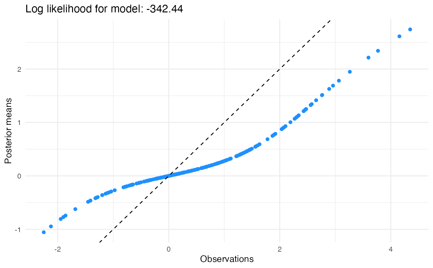
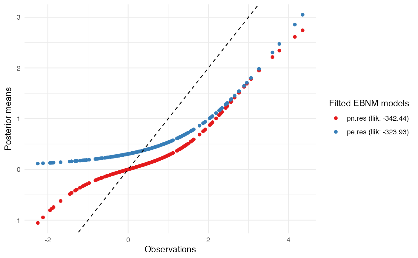
Given one or more fitted ebnm object(s), produces a plot of posterior means vs. observations. If desired, a plot of cumulative distribution functions of fitted prior(s) can also be produced.

# S3 method for ebnm
plot(
  x,
  ...,
  incl_pm = TRUE,
  incl_cdf = FALSE,
  subset = NULL,
  remove_abline = FALSE
)

Arguments

x

The fitted ebnm object.

...

Additional ebnm objects to be included on the same plots.

incl_pm

Plot posterior means vs. observations?

incl_cdf

Plot the cumulative distribution functions?

subset

The subset of observations to include on the plot of posterior means vs. observations. Can be a numeric vector corresponding to indices of observations to plot, or a character vector if observations are named. If subset = NULL then all observations will be plotted.

remove_abline

To better illustrate shrinkage effects, the plot of posterior means vs. observations includes the line \(y = x\) by default. If remove_abline = TRUE, then this line will not be drawn.

Examples

theta <- c(rep(0, 100), rexp(100))
theta[1:50] <- 0
s <- 1
x <- theta + rnorm(200, 0, s)
pn.res <- ebnm_point_normal(x, s)
plot(pn.res)


pe.res <- ebnm_point_exponential(x, s)
plot(pn.res, pe.res)


# Customize plot:
library(ggplot2)
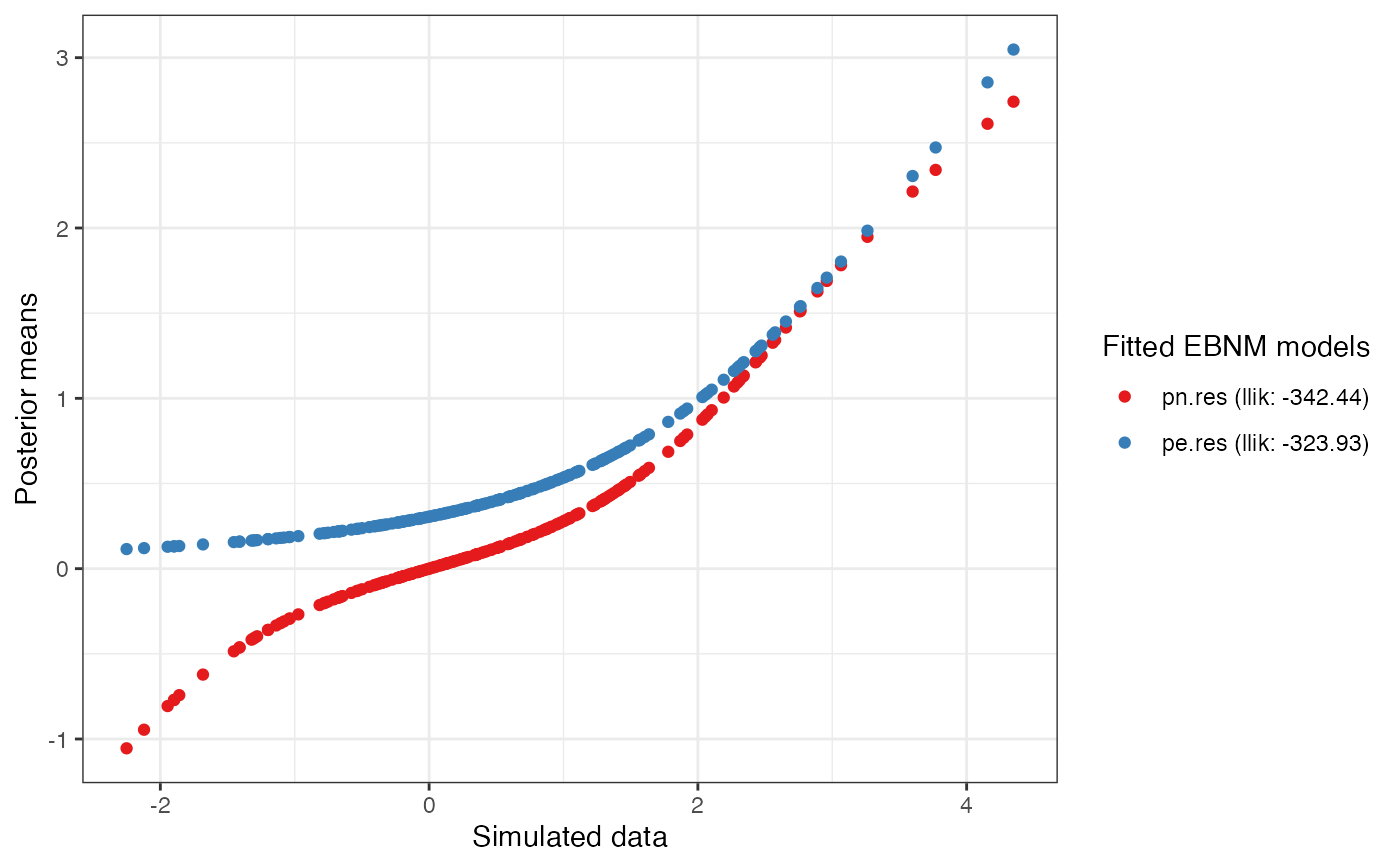
plot(pn.res, pe.res, remove_abline = TRUE) +
  theme_bw() +
  labs(x = "Simulated data")