An R example: ashr benchmark

This is a more advanced application of DSC with R scripts. We demonstrate in this tutorial features of DSC including:

• Inline code as parameters
• @ALIAS decorator
• R library installation and version check
• Use dscrutils to query results limited to given conditions

DSC Problem

The DSC problem is based on the ASH example of DSCR (R Markdown version and HTML version). Material to run this tutorial can be found in DSC vignettes repo. Description below is copied from the DSCR vignette:

To illustrate we consider the problem of shrinkage, which is tackled by the ashr package at http://www.github.com/stephens999/ashr. The input to this DSC is a set of estimates $\hat\beta$, with associated standard errors $s$. These values are estimates of actual (true) values for $\beta$, so the meta-data in this case are the true values of beta. Methods must take $\hat\beta$ and $s$ as input, and provide as output “shrunk” estimates for $\beta$ (so output is a list with one element, called beta_est, which is a vector of estimates for beta). The score function then scores methods on their RMSE comparing beta_est with beta.

First define a datamaker which simulates true values of $\beta$ from a user-specified normal mixture, where one of the components is a point mass at 0 of mass $\pi_0$, which is a user-specified parameter. It then simulates $\hat\beta \sim N(\beta_j,s_j)$ (where $s_j$ is again user-specified). It returns the true $\beta$ values and true $\pi_0$ value as meta-data, and the estimates $\hat\beta$ and $s$ as input-data.

Now define a method wrapper for the ash function from the ashr package. Notice that this wrapper does not return output in the required format - it simply returns the entire ash output.

Finally add a generic (can be used to deal with both $\pi$ and $\beta$) score function to evaluate estimates by ash.

DSC Specification

The problem is fully specified in DSC syntax below, following the structure of the original DSCR implementation:

#!/usr/bin/env dsc
simulate: datamaker.R
    # module input and variables
    mixcompdist: normalmix
    g: (c(2/3,1/3),c(0,0),c(1,2)),
       (rep(1/7,7),c(-1.5,-1,-0.5,0,0.5,1,1.5),rep(0.5,7)),
       (c(1/4,1/4,1/3,1/6),c(-2,-1,0,1),c(2,1.5,1,1))
    min_pi0: 0
    max_pi0: 1
    nsamp: 1000
    betahatsd: 1
    # module decoration
    @ALIAS: args = List()
    # module output
    $data: data
    $true_beta: data$meta$beta
    $true_pi0: data$meta$pi0

shrink: runash.R
    # module input and variables
    data: $data
    mixcompdist: "normal", "halfuniform"
    # module output
    $ash_data: ash_data
    $beta_est: ashr::get_pm(ash_data)
    $pi0_est: ashr::get_pi0(ash_data)

score_beta: score.R
    # module input and variables
    est: $true_beta
    truth: $beta_est
    # module output aka pipeline variable
    $mse: result

score_pi0: score.R
    # module input and variables
    est: $pi0_est
    truth: $true_pi0
    # module output
    $mse: result

DSC:
    # module ensembles
    define:
      score: score_beta, score_pi0
    # pipelines
    run: simulate * shrink * score
    # runtime environments
    R_libs: ashr@stephens999 (2.2.7+)
    exec_path: bin
    output: dsc_result

It is suggested that you check out the corresponding R codes for modules simulate, shrink and the score function to figure out how DSC communicates with your R scripts.

Here we will walk through all modules to highlight important syntactical elements.

Module simulate

Un-quoted string as parameters and output values

The parameter g has three candidate values, all of which are un-quoted string to be plugged to script as is. In other words, DSC will interpret each as, eg, g <- list(c(2/3,1/3),c(0,0),c(1,2)) so that g will be assigned at runtime the output of R codes as specified for use with datamaker.R. Similarly, mixcompdist: normalmix will be interpreted as mixcompdist <- normalmix – this statement is valid as long as datamaker.R has loaded ashr library, because normalmix is function from ashr library.

Decorator @ALIAS for R list

Inside datamaker.R the input for the core function is a single parameter of an R list containing all parameters specified in this module. The decorator @ALIAS uses a special DSC operation List() to consolidate these parameters into an R list args which corresponds to the input parameter in datamaker.R.

Module shrink

Here notice the output variable are also provided at runtime: DSC allows output variables to directly accept pieces of codes that can provide the desired output. In this case, get_pi0 function from ashr package will get us what we need.

Module beta_score & pi0_score

These modules uses the same module executable score.R but on different input data. Due to differences in variable names it makes sense to configure them in separate blocks. However an alternative style that configures them in the same block is:

score_beta, score_pi0: score.R
    @score_beta:
        est: $true_beta
        truth: $beta_est
        $mse_beta: result
    @score_pi0:
        est: $pi0_est
        truth: $true_pi0
        $mse_pi: result        

Here @* are module specific variable decorations that configures input and output such that different modules can be allowed in the same block.

Notice that different from the DSCR ASH example the output score is an “atomic” value (a float number). If the outcome object result is not such a simple object, for example it returns an R list, then you may want to code it to only extract the information you need so that they’ll be readily extractable in the benchmark query process – the query process can only extract atomic types. To do so, you can write something like, e.g., $mse_pi: score_output$mse.

DSC section for benchmark configuration

As has been discussed in previous tutorials, DSC sections defines module / pipeline ensembles and a benchmark. This DSC executes essentially two pipelines (one ending with score_beta another with score_pi0). The R_libs property specifies the R package required by the DSC. It is formatted as a github package (pkg@repo) and the minimal version requirement is 2.0.0. DSC will check first if the package is available and up-to-date, and install it if necessary. It will then check its version and quit on error if it does not satisfy the requirement. For safety concerns, DSC does not attempt to upgrade/downgrade a package in cases of version mismatch.

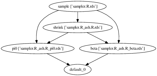
Execution logic

This diagram (generated by dot command using execution graph of this DSC) shows the logic of the benchmark:

Run DSC

We now run this DSC with 10 replicates:

cd ~/GIT/dsc/vignettes/ash

./settings.dsc --replicate 10

INFO: Checking R library ashr@stephens999/ashr ...
INFO: Checking R library dscrutils@stephenslab/dsc/dscrutils ...
INFO: DSC script exported to dsc_result.html
INFO: Constructing DSC from ./settings.dsc ...
INFO: Building execution graph & running DSC ...
[#########] 9 steps processed (215 jobs completed)
INFO: Building DSC database ...
INFO: DSC complete!
INFO: Elapsed time 85.268 seconds.

Benchmark evaluation

Extract result of interest

The DSCR ASH example has names to various simulation settings and methods. Here we use dscrutils to reproduce the DSCR example. It is similar to what we have done in the DSC Introduction example, but we will demonstrate the use of condition argument, to create 3 data-sets:

setwd('~/GIT/dsc/vignettes/ash')
dsc_dir = 'dsc_result'

An = dscrutils::dscquery(dsc_dir, targets = c("simulate.true_pi0",
                                              "shrink.mixcompdist",
                                              "shrink.beta_est",
                                              "shrink.pi0_est",
                                              "score.mse"),
                         condition = "simulate.g = 'list(c(2/3,1/3),c(0,0),c(1,2))'")

Loading dsc-query output from CSV file.
Reading DSC outputs:
 - simulate.true_pi0: extracted atomic values
 - shrink.beta_est: vectors not extracted (set max.extract.vector = 1000 to extract)
 - shrink.pi0_est: extracted atomic values
 - score.mse: extracted atomic values

Bn = dscrutils::dscquery(dsc_dir, targets = c("simulate.true_pi0",
                                              "shrink.mixcompdist",
                                              "shrink.beta_est",
                                              "shrink.pi0_est", 
                                              "score.mse"),
                         condition = "simulate.g = 'list(rep(1/7,7),c(-1.5,-1,-0.5,0,0.5,1,1.5),rep(0.5,7))'")

Loading dsc-query output from CSV file.
Reading DSC outputs:
 - simulate.true_pi0: extracted atomic values
 - shrink.beta_est: vectors not extracted (set max.extract.vector = 1000 to extract)
 - shrink.pi0_est: extracted atomic values
 - score.mse: extracted atomic values

Cn = dscrutils::dscquery(dsc_dir, targets = c("simulate.true_pi0",
                                              "shrink.mixcompdist",
                                              "shrink.beta_est",
                                              "shrink.pi0_est", 
                                              "score.mse"),
                         condition = "simulate.g = 'list(c(1/4,1/4,1/3,1/6),c(-2,-1,0,1),c(2,1.5,1,1))'")

Loading dsc-query output from CSV file.
Reading DSC outputs:
 - simulate.true_pi0: extracted atomic values
 - shrink.beta_est: vectors not extracted (set max.extract.vector = 1000 to extract)
 - shrink.pi0_est: extracted atomic values
 - score.mse: extracted atomic values

To view one of the resulting data frame:

head(An)

Explore results of interest

Suppose we are interested in comparing $\pi_0$ estimates under scenario An, for two flavors of shrink module normal and halfuniform.

normal = subset(An, shrink.mixcompdist == 'normal')
hu = subset(An, shrink.mixcompdist == 'halfuniform')

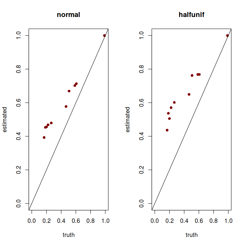
First, we visualize estimated vs true $\pi_0$ for two methods:

par(mfrow=c(1,2))
plot(subset(normal, score == 'score_pi0')$simulate.true_pi0, 
     subset(normal, score == 'score_pi0')$shrink.pi0_est, 
     xlab = 'truth', ylab = 'estimated', main = 'normal', 
     pch = 16, col = "#800000", xlim = c(0,1), ylim = c(0,1))
abline(a=0,b=1)
plot(subset(hu, score == 'score_pi0')$simulate.true_pi0, 
     subset(hu, score == 'score_pi0')$shrink.pi0_est, 
     xlab = 'truth', ylab = 'estimated', main = 'halfunif', 
     pch = 16, col = "#800000", xlim = c(0,1), ylim = c(0,1))
abline(a=0,b=1)

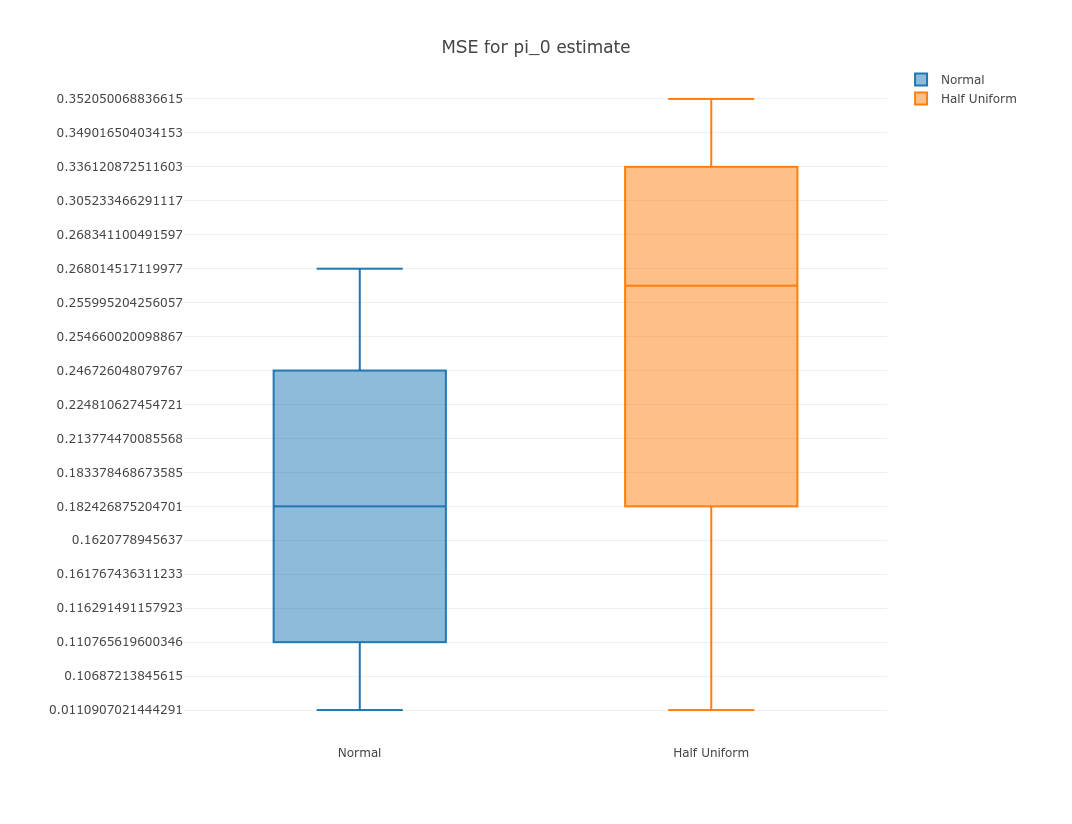
We then summarize the MSE scores for the two methods:

suppressMessages(library(plotly))
options(warn=-1)
p = plot_ly(y = subset(normal, score == 'score_pi0')$score.mse, name = 'Normal', type = "box") %>%
    add_trace(y = subset(hu, score == 'score_pi0')$score.mse, name = 'Half Uniform', type = "box")  %>% 
    layout(title = "MSE for pi_0 estimate")

export(p, file = 'mse.png')
IRdisplay::display_png(file="mse.png")

Explore intermediate output

We have previously focused on benchmark “results”, ie, the mean square errors. It is also possible to extract quantities of interest from any module in the benchmark. For example we want to explore relationship between “true” value and posterior estimates of $\beta$ from method normal and halfnormal. First we use dscrutils to extract these quantities:

dat2 = dscrutils::dscquery(dsc_dir,
                           targets = c("simulate.true_beta", "shrink.mixcompdist", "shrink.beta_est"),
                           condition = "simulate.g = 'list(c(2/3,1/3),c(0,0),c(1,2))'",
                           max.extract.vector = 1000)

Loading dsc-query output from CSV file.
Reading DSC outputs:
 - simulate.true_beta: extracted vector values
 - shrink.beta_est: extracted vector values

print(dim(dat2))

[1]   20 2002

head(dat2[,1:5])

As shown above, with max.extract.vector = 1000 we allow for extracting vector-valued $\beta$ estimates into the outputted data frame. The resulting dataframe has 2001 columns containing both $\beta$ and its posterior estimate $\tilde{\beta}{\text{normal}}$ and $\tilde{\beta}{\text{halfunif}}$. We make them into separate tables. Rows in each table are replicates.

pattern = "simulate.true_beta"
cols = which(sapply(strsplit(names(dat2),"[.]"), function (x) paste0(x[1],'.', x[2])) == pattern)
normal0 = subset(dat2, shrink.mixcompdist == 'normal')[,cols]
hu0 = subset(dat2, shrink.mixcompdist == 'halfuniform')[,cols]                 
#
pattern = "shrink.beta_est"
cols = which(sapply(strsplit(names(dat2),"[.]"), function (x) paste0(x[1],'.', x[2])) == pattern)
normal = subset(dat2, shrink.mixcompdist == 'normal')[,cols]
hu = subset(dat2, shrink.mixcompdist == 'halfuniform')[,cols]             

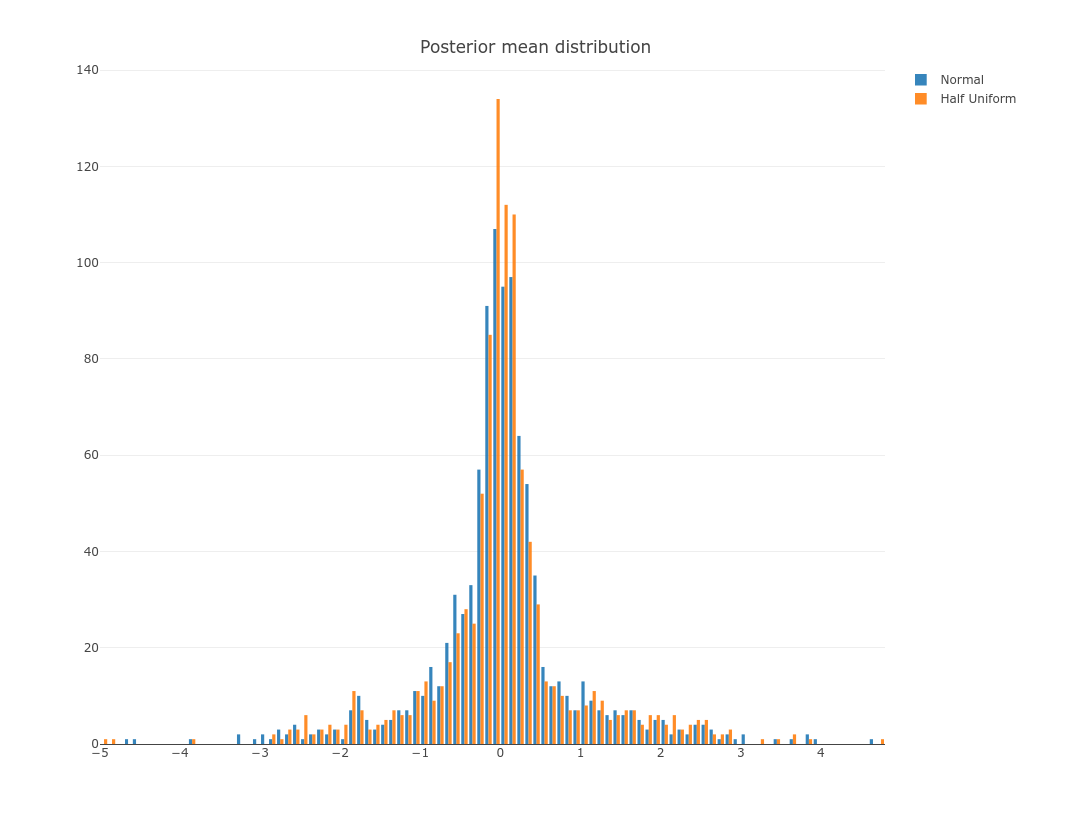
To view distribution of $\tilde{\beta}$ from one replicate:

p = plot_ly(x = as.numeric(normal[1,]), name = 'Normal', opacity = 0.9, type = "histogram") %>%
  add_trace(x = as.numeric(hu[1,]), name = 'Half Uniform', opacity = 0.9, type = "histogram") %>%
  layout(title = "Posterior mean distribution")

export(p, file = 'beta.png')
IRdisplay::display_png(file="beta.png")

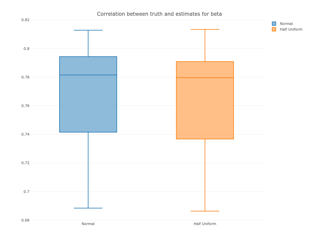
Now we compare correlation between estimate and the truth for these 2 methods:

normal0 = as.matrix(normal0)
normal = as.matrix(normal)
normal_cor = sapply(seq.int(dim(normal0)[1]), function(i) cor(normal0[i,], normal[i,]))

hu0 = as.matrix(hu0)
hu = as.matrix(hu)
hu_cor = sapply(seq.int(dim(hu0)[1]), function(i) cor(hu0[i,], hu[i,]))

p = plot_ly(y = normal_cor, name = 'Normal', type = "box") %>%
    add_trace(y = hu_cor, name = 'Half Uniform', type = "box")  %>% 
    layout(title = "Correlation between truth and estimates for beta")

export(p, file = 'corr.png')
IRdisplay::display_png(file="corr.png")