Attempt at Automating SuSiE for Hard Problems

susie_auto is an attempt to automate reliable running of susie even on hard problems. It implements a three-stage strategy for each L: first, fit susie with very small residual error; next, estimate residual error; finally, estimate the prior variance. If the last step estimates some prior variances to be zero, stop. Otherwise, double L, and repeat. Initial runs are performed with relaxed tolerance; the final run is performed using the default susie tolerance.

Usage

susie_auto(
  X,
  y,
  L_init = 1,
  L_max = 512,
  verbose = FALSE,
  init_tol = 1,
  standardize = TRUE,
  intercept = TRUE,
  max_iter = 100,
  tol = 0.01,
  ...
)

Arguments

X

An n by p matrix of covariates.

y

The observed responses, a vector of length n.

L_init

The initial value of L.

L_max

The largest value of L to consider.

verbose

If verbose = TRUE, the algorithm's progress, and a summary of the optimization settings, are printed to the console.

init_tol

The tolerance to passed to susie during early runs (set large to shorten the initial runs).

standardize

If standardize = TRUE, standardize the columns of X to unit variance prior to fitting. Note that scaled_prior_variance specifies the prior on the coefficients of X after standardization (if it is performed). If you do not standardize, you may need to think more carefully about specifying scaled_prior_variance. Whatever your choice, the coefficients returned by coef are given for X on the original input scale. Any column of X that has zero variance is not standardized.

intercept

If intercept = TRUE, the intercept is fitted; it intercept = FALSE, the intercept is set to zero. Setting intercept = FALSE is generally not recommended.

max_iter

Maximum number of IBSS iterations to perform.

tol

A small, non-negative number specifying the convergence tolerance for the IBSS fitting procedure. The fitting procedure will halt when the difference in the variational lower bound, or “ELBO” (the objective function to be maximized), is less than tol.

...

Additional arguments passed to susie.

Value

See susie for a description of return values.

See also

susie

Examples

set.seed(1)
n = 1000
p = 1000
beta = rep(0,p)
beta[1:4] = 1
X = matrix(rnorm(n*p),nrow = n,ncol = p)
X = scale(X,center = TRUE,scale = TRUE)
y = drop(X %*% beta + rnorm(n))
res = susie_auto(X,y)
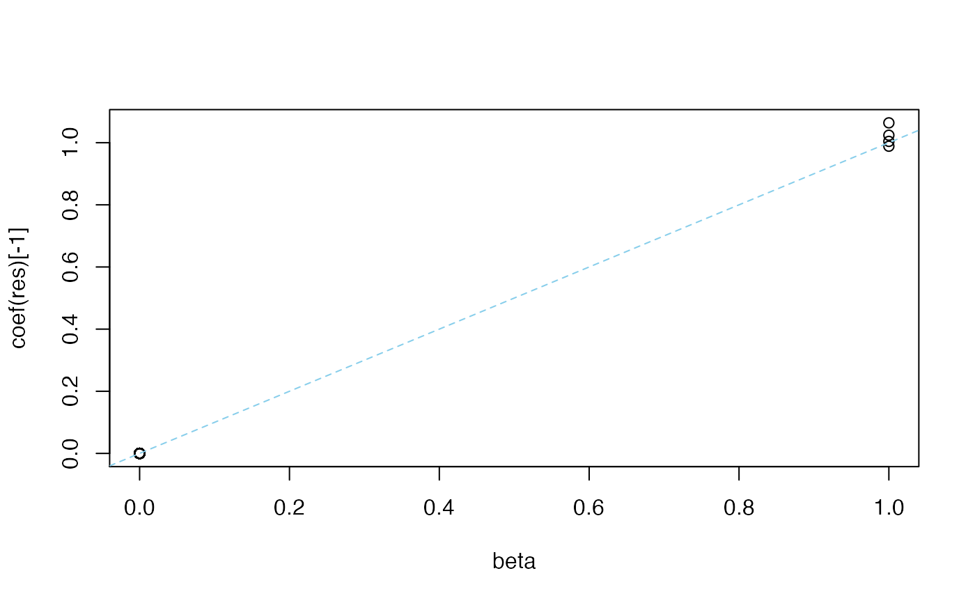
plot(beta,coef(res)[-1])
abline(a = 0,b = 1,col = "skyblue",lty = "dashed")

plot(y,predict(res))
abline(a = 0,b = 1,col = "skyblue",lty = "dashed")