Trend filtering
Matthew Stephens
2026-05-01
Source:vignettes/trend_filtering.Rmd
trend_filtering.RmdIntroduction
Although we developed SuSiE primarily with the goal of performing variable selection in highly sparse settings – and, in particular, for genetic fine-mapping – the approach also has considerable potential for application to other large-scale regression problems. Here we briefly illustrate this potential by applying it to a non-parametric regression problem that at first sight seems to be ill-suited to our approach. In particular, it does not involve strict sparsity, and the underlying correlation structure of the explanatory variables is very different from the “blocky” covariance structure of genetic data that SuSiE was designed for. Nonetheless, we will see that SuSiE performs well here despite this (partly due to its ability to capture non-sparse signals via Bayesian Model Averaging).
Specifically, consider the non-parametric regression: y_t = \mu_t + e_t \quad t=1,\dots,T where the goal is to estimate the underlying mean, \mu_t, under the assumption that it varies smoothly (or, more precisely, in a spatially-structured way) with t. One very simple way to capture spatial structure in \mu is to model it as a (sparse) linear combination of step functions: \mu = Xb where the jth column of X is the step function with a step at j (j = 1,\dots,(T-1)); that is x_{tj}=0 for t<=j and 1 for t>j. The jth element of b therefore determines the change in the mean |\mu_j-\mu_{j+1}|, and an assumption that b is sparse encapsulates an assumption that \mu is spatially structured (indeed, piecewise constant).
This very simple approach is essentially 0th-order trend filtering (Tibshirani, 2014, Annals of Statistics 42, 285–323). Note that higher-order trend filtering can be similarly implemented using different basis functions; here we use 0th order only for simplicity.
Examples
Here we apply SuSiE to perform 0th order trend filtering in some
simple simulated examples. We have implemented in susieR
0.6.0 a funciton susie_trendfilter which internally creates
X matrix with step functions in the
columns to match input y. The algebra
have been optimized to work on such trendfiltering matrices. Here we
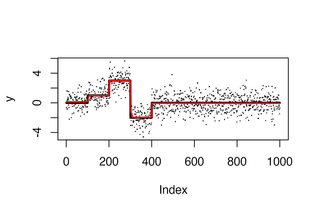
simulate some data where \mu is a step
function with four steps, a 0th order trendfiltering problem. The
regression is truly sparse and SuSiE should do well.
library(susieR)
set.seed(1)
n=1000
mu = c(rep(0,100),rep(1,100),rep(3,100),rep(-2,100),rep(0,600))
y = mu + rnorm(n)
s = susie_trendfilter(y, 0, L=10)
# WARNING: IBSS algorithm did not converge in 100 iterations!
# WARNING: IBSS algorithm did not converge in 100 iterations!
Plot results: the truth is black, and susie estimate is red.

s$sigma2
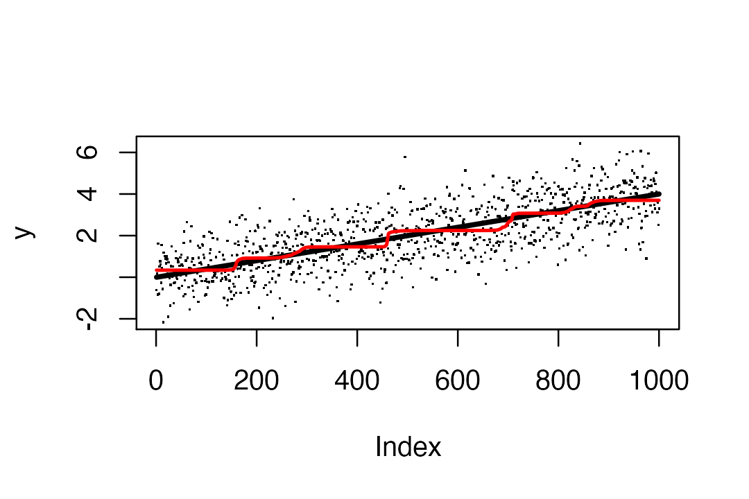
# [1] 1.076261In the next example mu increases linearly. Thus we are approximating a linear function by step functions. Here the truth is not trully “sparse”, so we might expect performance to be poor, but it is not too bad.
set.seed(1)
mu = seq(0,4,length=1000)
y = mu + rnorm(n)
s = susie_trendfilter(y,0,L=10)
plot(y,pch=".")
lines(mu,col=1,lwd=3)
lines(predict(s),col=2,lwd=2)
Compare with the genlasso (lasso-based) solution (blue). (This will
require installation of the genlasso package, which is not
available on CRAN, but can be installed from GitHub.)
# install.packages("remotes")
# remotes::install_github("glmgen/genlasso")
y.tf = trendfilter(y,ord=0)
y.tf.cv = cv.trendfilter(y.tf)
plot(y,pch=".")
lines(mu,col=1,lwd=3)
lines(predict(s),col=2,lwd=2)
lines(y.tf$fit[,which(y.tf$lambda==y.tf.cv$lambda.min)],col=4,lwd=2)
What happens if we have linear trend plus a sudden change.
set.seed(1)
mu = seq(0,4,length=1000)
mu = mu + c(rep(0,500),rep(4,500))
y = mu + rnorm(n)
s = susie_trendfilter(y,0,L=10)
y.tf = trendfilter(y,ord=0)
y.tf.cv = cv.trendfilter(y.tf)
plot(y,pch=".")
lines(mu,col=1,lwd=3)
lines(predict(s),col=2,lwd=2)
lines(y.tf$fit[,which(y.tf$lambda==y.tf.cv$lambda.min)],col=4,lwd=2)
The two fits seem similar in accuracy. We can check this numerically: