Sparse matrix multiplication strategy
Kaiqian Zhang
2021-08-29
Source:vignettes/sparse_matrix_strategy.Rmd
sparse_matrix_strategy.RmdGeneral strategy
Given a large sparse matrix X, we want to compute some matrix multiplications associated with a scaled \(\tilde{X}\). We notice that after scaling, X becomes a dense matrix and is not possible for a sparse matrix multiplication. So we construct formulae to apply sparse matrix multiplication first on a standardized X since standardization does not affect its sparsity. Then we perform centering to get the same result.
Types of matrix multiplications
There are two types of matrix multiplications we want to investigate:
Compute \(\tilde{X}b\), where \(\tilde{X}\) is an n by p scaled matrix and \(b\) is a p vector.
Compute \(\tilde{X}^Ty\), where \(\tilde{X}\) is an n by p scaled matrix and \(y\) is an n vector.
Results
This strategy has a decent performance when computing both \(\tilde{X}b\) and \(\tilde{X}^Ty\), compared to simple matrix multiplication %*%.
Strategy formulae details
Computing \(\boldsymbol{\tilde{X}b}\)
Suppose we want to compute \(\tilde{X}b\), where \(\tilde{X}\) is a scaled n by p matrix and \(b\) is a p vector. Our goal is to express \(\tilde{X}b\) into a term involving unscaled \(X\) matrix multiplication to achieve sparse matrix operation.
\[\begin{equation} \begin{aligned} \tilde{X}b &= \sum_{j=1}^{p} \tilde{X}_{\cdot j} b_j \\ &= \sum_{j=1}^{p} \frac{X_{\cdot j}-\mu_j}{\sigma_j}b_j \\ &= \sum_{j=1}^{p}\frac{X_{\cdot j}}{\sigma_j}b_j - \sum_{j=1}^{p} \frac{\mu_j}{\sigma_j}b_j \\ &= X b / \sigma - \mu^Tb/\sigma, \end{aligned} \end{equation}\]
where \(\mu\) is a p-vector of column means, and \(\sigma\) is a p-vector of column standard deviations.
Computing \(\boldsymbol{\tilde{X}^Ty}\)
Suppose we want to compute \(\tilde{X}^Ty\), where \(\tilde{X}\) is a scaled n by p matrix and \(y\) is an n vector. Similarly, we express \(\tilde{X}^Ty\) using unscaled \(X\) so that we can perform sparse matrix multiplication. We have the following:
\[\begin{equation} \begin{aligned} \tilde{X}^Ty &= \sum_{i=1}^{n} \tilde{X}_{i.}y_i \\ &= \sum_{i=1}^{n} \frac{X_{i.} - \mu}{\sigma}y_i \\ &= \frac{1}{\sigma}\sum_{i=1}^{n}X_{i.}y_i - \frac{\mu}{\sigma}\sum_{i=1}^{n} y_i \\ &= \frac{1}{\sigma}(X^Ty) - \frac{\mu}{\sigma}y^T 1, \end{aligned} \end{equation}\]
where \(\mu\) is a p-vector of column means, and \(\sigma\) is a p-vector of columnwise standard deviations.
Simulations
We simulate an n = 1000 by p = 10000 matrix X at sparsity \(99\%\), i.e. \(99\%\) entries are zeros. We compare results between normal matrix computation and our sparse strategy as well as comparing speed using microbenchmark.
create_sparsity_mat <- function(sparsity, n, p) {
  nonzero          <- round(n*p*(1-sparsity))
  nonzero.idx      <- sample(n*p, nonzero)
  mat              <- numeric(n*p)
  mat[nonzero.idx] <- 1
  mat              <- matrix(mat, nrow=n,ncol=p)
  return(mat)
}
n <- 1000
p <- 10000
X.dense  <- create_sparsity_mat(0.99,n,p)
X.sparse <- as(X.dense,"dgCMatrix")
X.tilde  <- susieR:::set_X_attributes(X.dense) #returns a scaled X if input is a dense matrix
X <- susieR:::set_X_attributes(X.sparse) #return an unsacled sparse X if input is a sparse matrix
#but computes column means and standard deviationsBenchmark for computing \(\boldsymbol{\tilde{X}b}\)
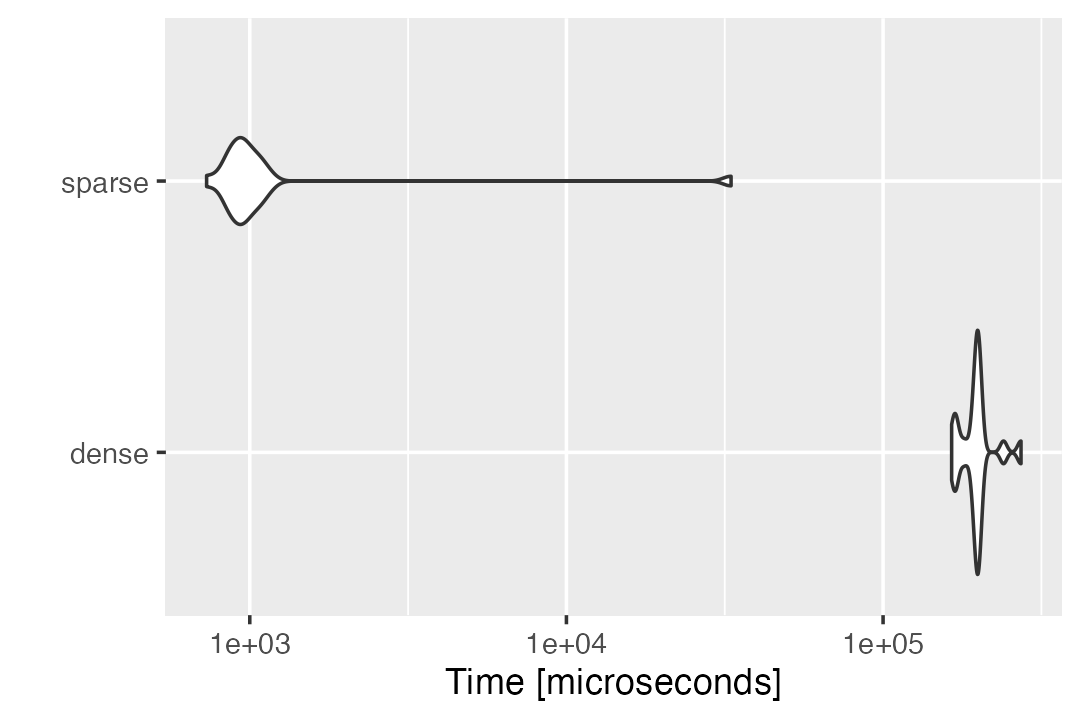
The final results of two methods when computing \(\tilde{X}b\) are very close.
compute_Xb_benchmark <- microbenchmark(
  dense  = (use.normal.Xb <- X.tilde%*%b),
  sparse = (use.sparse.Xb <- susieR:::compute_Xb(X,b)),
  times = 20,unit = "s")
Our sparse strategy demonstrates an obvious advantage over the normal matrix multiplication in computing \(\tilde{X}b\).
autoplot(compute_Xb_benchmark)
# Coordinate system already present. Adding new coordinate system, which will replace the existing one.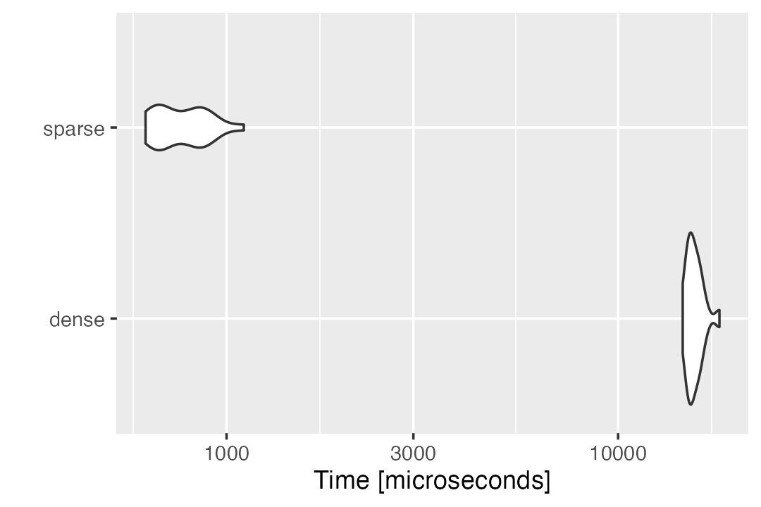
Benchmark for computing \(\boldsymbol{\tilde{X}^Ty}\)
The final results of two methods when computing \(\tilde{X}^Ty\) are almost the same.
compute_Xty_benchmark = microbenchmark(
  dense  = (use.normal.Xty <- t(X.tilde)%*%y),
  sparse = (use.sparse.Xty <- susieR:::compute_Xty(X, y)),
  times = 20,unit = "s")
Our sparse strategy evidently has a better performance than the normal method in computing \(\tilde{X}^Ty\).
autoplot(compute_Xty_benchmark)
# Coordinate system already present. Adding new coordinate system, which will replace the existing one.