Exploring Cicero co-assessibility data in kidney data
Peter Carbonetto
Last updated: 2022-08-31
Checks: 7 0
Knit directory: scATACseq-topics/
This reproducible R Markdown analysis was created with workflowr (version 1.7.0). The Checks tab describes the reproducibility checks that were applied when the results were created. The Past versions tab lists the development history.
Great! Since the R Markdown file has been committed to the Git repository, you know the exact version of the code that produced these results.
Great job! The global environment was empty. Objects defined in the global environment can affect the analysis in your R Markdown file in unknown ways. For reproduciblity it’s best to always run the code in an empty environment.
The command set.seed(20200729) was run prior to running
the code in the R Markdown file. Setting a seed ensures that any results
that rely on randomness, e.g. subsampling or permutations, are
reproducible.
Great job! Recording the operating system, R version, and package versions is critical for reproducibility.
Nice! There were no cached chunks for this analysis, so you can be confident that you successfully produced the results during this run.
Great job! Using relative paths to the files within your workflowr project makes it easier to run your code on other machines.
Great! You are using Git for version control. Tracking code development and connecting the code version to the results is critical for reproducibility.
The results in this page were generated with repository version d9555fc. See the Past versions tab to see a history of the changes made to the R Markdown and HTML files.
Note that you need to be careful to ensure that all relevant files for
the analysis have been committed to Git prior to generating the results
(you can use wflow_publish or
wflow_git_commit). workflowr only checks the R Markdown
file, but you know if there are other scripts or data files that it
depends on. Below is the status of the Git repository when the results
were generated:
Ignored files:
    Ignored:    .DS_Store
    Ignored:    data/.DS_Store
    Ignored:    data/Buenrostro_2018/
    Ignored:    data/Cusanovich_2018/processed_data/Cusanovich_2018_Kidney.RData
    Ignored:    output/Buenrostro_2018/binarized/filtered_peaks/de-buenrostro2018-k=10-noshrink.RData
    Ignored:    output/Buenrostro_2018/binarized/filtered_peaks/fit-Buenrostro2018-binarized-filtered-scd-ex-k=10.rds
    Ignored:    output/Buenrostro_2018/binarized/filtered_peaks/fit-Buenrostro2018-binarized-filtered-scd-ex-k=8.rds
    Ignored:    output/Cusanovich_2018/
    Ignored:    scripts/seq_gene.md.gz

Untracked files:
    Untracked:  analysis/fit-Buenrostro2018-binarized-scd-ex-k=10.rds
    Untracked:  data/Buenrostro_2018_binarized.RData
    Untracked:  output/Buenrostro_2018/binarized/filtered_peaks/Buenrostro_2018_binarized_filtered.RData
    Untracked:  plots/
    Untracked:  scripts/fit-buenrostro-2018-k=8.rds
Note that any generated files, e.g. HTML, png, CSS, etc., are not included in this status report because it is ok for generated content to have uncommitted changes.
These are the previous versions of the repository in which changes were
made to the R Markdown (analysis/explore_cicero.Rmd) and
HTML (docs/explore_cicero.html) files. If you’ve configured
a remote Git repository (see ?wflow_git_remote), click on
the hyperlinks in the table below to view the files as they were in that
past version.
| File | Version | Author | Date | Message |
|---|---|---|---|---|
| Rmd | d9555fc | Peter Carbonetto | 2022-08-31 | workflowr::wflow_publish("explore_cicero.Rmd") |
| Rmd | 0d848fc | Peter Carbonetto | 2022-08-30 | Implemented initial steps of gene_scores_cusanovich2018_kidney_k10.R script. |
| html | 93cb793 | Peter Carbonetto | 2022-08-30 | Added scatterplot showing LFC estimates before vs. after ash. |
| Rmd | e931791 | Peter Carbonetto | 2022-08-30 | workflowr::wflow_publish("analysis/explore_cicero.Rmd", verbose = TRUE) |
| html | 69df48d | Peter Carbonetto | 2022-08-30 | Added more text to explore_cicero analysis. |
| Rmd | 22bb834 | Peter Carbonetto | 2022-08-30 | workflowr::wflow_publish("analysis/explore_cicero.Rmd", verbose = TRUE) |
| Rmd | 84c54c8 | Peter Carbonetto | 2022-08-29 | A couple small improvements to the explore_cicero analysis. |
| Rmd | 89de024 | Peter Carbonetto | 2022-08-29 | Adding another plot to the explore_cicero analysis. |
| html | ff33f2d | Peter Carbonetto | 2022-08-29 | Added scatterplot to explore_cicero analysis. |
| Rmd | d1f8485 | Peter Carbonetto | 2022-08-29 | workflowr::wflow_publish("analysis/explore_cicero.Rmd") |
| Rmd | 7f6b8a5 | Peter Carbonetto | 2022-08-29 | Added steps to explore_cicero analysis to load topic model fit and de_analysis results. |
| Rmd | ac066af | Peter Carbonetto | 2022-08-29 | Added some text to the explore_cicero analysis. |
| html | 83686bc | Peter Carbonetto | 2022-08-29 | First build of the explore_cicero workflowr analysis. |
| Rmd | 522f408 | Peter Carbonetto | 2022-08-29 | workflowr::wflow_publish("analysis/explore_cicero.Rmd") |
| Rmd | 39fecb3 | Peter Carbonetto | 2022-08-29 | workflowr::wflow_publish("analysis/index.Rmd") |
The aim of this short analysis is to get a better understanding of the Cicero co-accessibility data, and how (and whether) these data can be used to connect chromatin accessibility peaks to genes in order to identify “driving genes” for topics estimated from single-cell ATAC-seq data. As an illustration, here we focus on the Cicero data for a single gene, Slc12a1, that was highlighted in Cusanovich et al, 2018 in connection with the “loop of henle” cell type (see Fig. 5 of that paper, and see also Park et al, 2018).
Load the packages used in the analysis below.
library(fastTopics)
library(ggplot2)
library(cowplot)
library(ashr)
Load the base-pair positions of the genes for the mm9 Mouse Genome Assembly.
load("data/mm9_seq_gene.RData")Load the Cicero co-accessibility data, including the “gene activity
scores”, for gene Slc12a1. (These data were downloaded from the
Mouse sci-ATAC-seq
Atlas website then prepared using the
extract_slc12a1_data.R script.)
load("data/Cusanovich_2018/processed_data/slc12a1_data.RData")
cicero <- transform(cicero,
                    Peak1 = as.character(Peak1),
                    Peak2 = as.character(Peak2))
Load the \(K = 10\) topic model fit, and the results of the DE analysis using this topic model (without the adaptive shrinkage step).
fit <- readRDS(file.path("output/Cusanovich_2018/tissues",
                         "fit-Cusanovich2018-Kidney-scd-ex-k=10.rds"))$fit
fit <- poisson2multinom(fit)
load(file.path("output/Cusanovich_2018/tissues",
               "de-cusanovich2018-kidney-k=10-noshrink.RData"))
From the Structure plots here, topic 8 appears to capture Loop of Henle (LoH) cells, so in the remainder we focus on topic 8.
k <- 8Get the base-pair positions of the peaks.
feature_names <- rownames(de$postmean)
out           <- strsplit(feature_names,"_")
positions     <- data.frame(chr   = sapply(out,"[[",1),
                            start = sapply(out,"[[",2),
                            end   = sapply(out,"[[",3),
                            name  = feature_names,
                            stringsAsFactors = FALSE)
positions <- transform(positions,
                       start = as.numeric(start),
                       end   = as.numeric(end))
Before examining the co-accessibility data in detail, this first plot confirms that Slc12a1 is highly relevant to topic 8, the LoH topic. It is a simple scatterplot showing the Slc12a1 gene activity score and topic proportion for each cell. The dashed blue line shows the “best fit” line between the two quantities. (Note that the gene activity scores are shown on the log-scale.)
pdat <- data.frame(loading = fit$L[,k],score = log10(1 + scores))
b <- coef(lm(score ~ loading,data = pdat))
ggplot(pdat,aes(x = loading,y = score)) +
  geom_point() +
  geom_abline(intercept = b["(Intercept)"],slope = b["loading"],
              color = "dodgerblue",size = 1,linetype = "dashed") +
  labs(x = "topic proportion",y = "gene activity score") +
  theme_cowplot()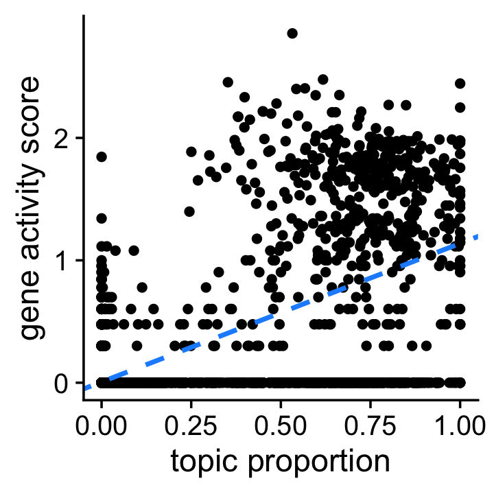
| Version | Author | Date |
|---|---|---|
| ff33f2d | Peter Carbonetto | 2022-08-29 |
THaving confirmed the strong relationship between Slc12a1
and topic 8, let’s examine more closely the de_analysis
results for the peaks near Slc12a1. Let’s use a window of 400
kb near the transcribed region of Slc12a1 (124.97–125.06 Mb on
chromosome 2).
d <- 4e5
seq_gene <- subset(seq_gene,feature_name == "Slc12a1")
rows <- which(with(positions,chr == paste0("chr",seq_gene$chromosome) &
                   start > seq_gene$chr_start - d &
                   end < seq_gene$chr_stop + d))
peaks <- c(cicero$Peak1,cicero$Peak2)
These next two plots show the p-values (top) and the LFC estimates for topic 8 and for the 111 peaks near Slc12a1. The peaks that are identified by Cicero as being relevant to Slc12a1 are highlighted in magenta.
pdat <- data.frame(start      = positions[rows,"start"]/1e5,
                   postmean   = de$postmean[rows,k],
                   z          = de$z[rows,k],
                   lpval      = de$lpval[rows,k],
                   cicero_hit = is.element(positions[rows,"name"],peaks))
p1 <- ggplot(pdat,aes(x = start,y = lpval,color = cicero_hit)) +
  geom_point() +
  scale_color_manual(values = c("royalblue","magenta")) +
  labs(x = "position on chromosome 2 (kb)",
       y = "-log10 p-value") +
  theme_cowplot()
p2 <- ggplot(pdat,aes(x = start,y = postmean,color = cicero_hit)) +
  geom_point() +
  geom_hline(yintercept = 0,color = "black",linetype = "dashed") +
  scale_color_manual(values = c("royalblue","magenta")) +
  labs(x = "position on chromosome 2 (kb)",
       y = "LFC estimate") +
  theme_cowplot()
plot_grid(p1,p2,nrow = 2,ncol = 1)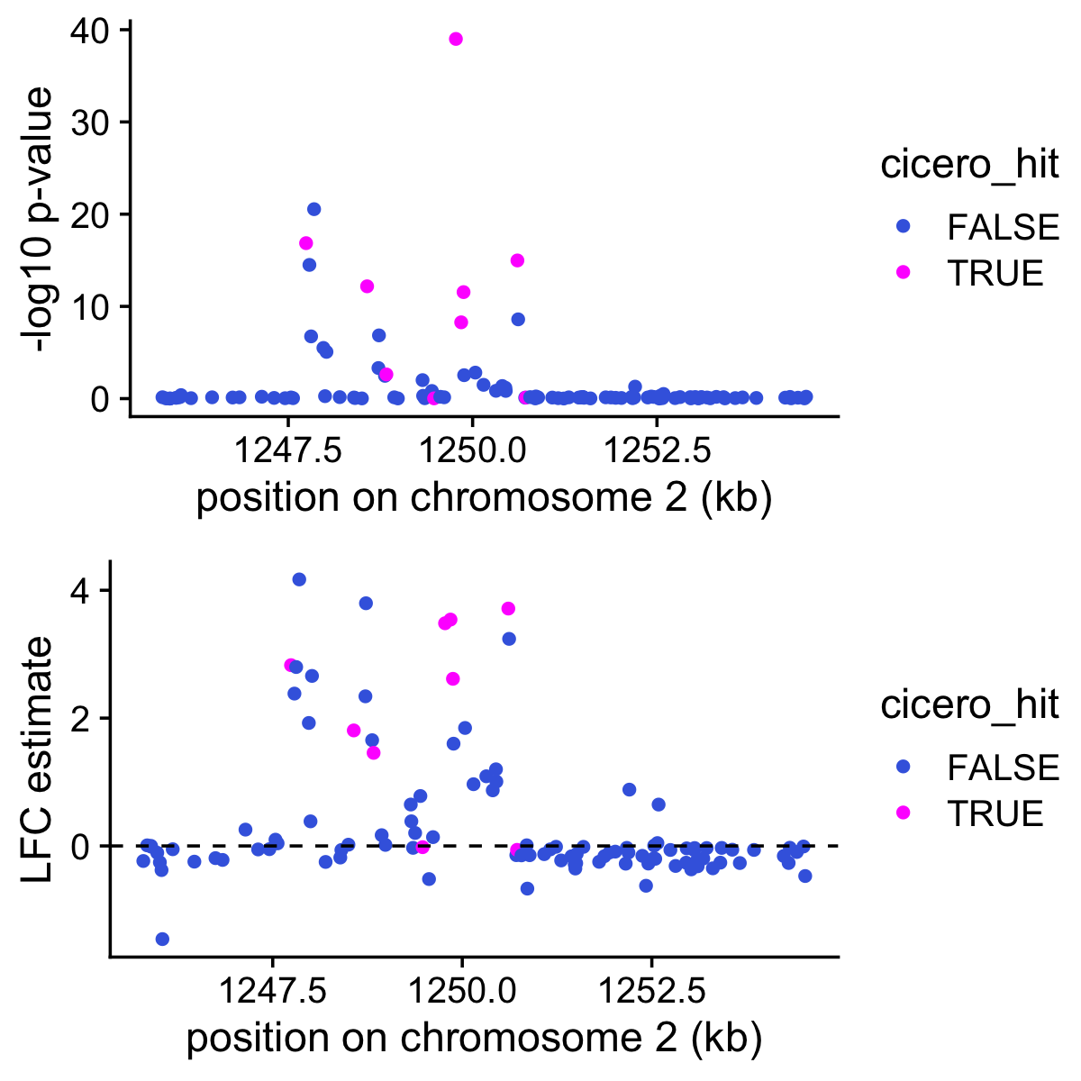
| Version | Author | Date |
|---|---|---|
| 69df48d | Peter Carbonetto | 2022-08-30 |
It is interesting that most of the Cicero-identified peaks show good evidence for being more accessible in topic 8. But it is also interesting that many other peaks near the gene also show good evidence for being more accessible in topic 8.
To improve the LFC estimates, a simple thing we can do is run ash separately on the subset of peaks that are near Slc12a1. By focussing on this small subset of peaks, ash should recognize that there is a strong signal near the gene, and not shrink the estimates too strongly.
pdat <- transform(pdat,se = postmean/z)
fit <- ash(pdat$postmean,pdat$se,mixcompdist = "normal",method = "shrink")
Indeed, ash preserves the strongest signals, and shrinks the others to zero, or close to zero. It is also interesting that the effects of all the Cicero-identified peaks remain after the adaptive shrinkage step:
pdat$ashmean <- fit$result$PosteriorMean
ggplot(pdat,aes(x = postmean,y = ashmean,color = cicero_hit)) +
  geom_point() +
  geom_abline(intercept = 0,slope = 1,color = "black",linetype = "dashed") +
  scale_color_manual(values = c("royalblue","magenta")) +
  labs(x = "original LFC estimate",y = "ash LFC estimate") +
  theme_cowplot()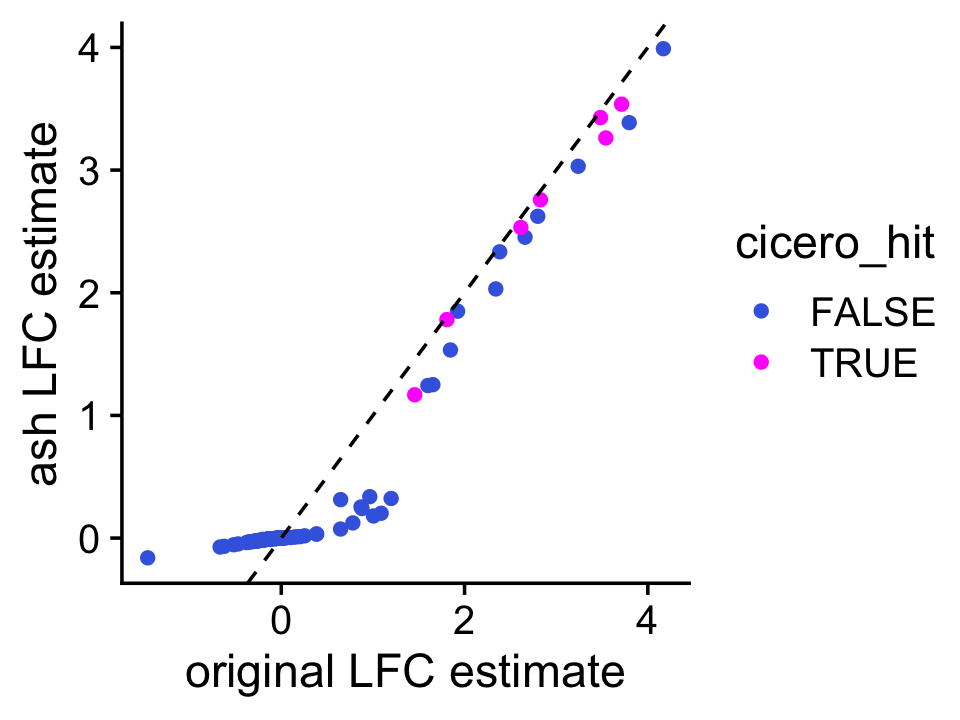
| Version | Author | Date |
|---|---|---|
| 93cb793 | Peter Carbonetto | 2022-08-30 |
sessionInfo()
# R version 3.6.2 (2019-12-12)
# Platform: x86_64-apple-darwin15.6.0 (64-bit)
# Running under: macOS Catalina 10.15.7
#
# Matrix products: default
# BLAS:   /Library/Frameworks/R.framework/Versions/3.6/Resources/lib/libRblas.0.dylib
# LAPACK: /Library/Frameworks/R.framework/Versions/3.6/Resources/lib/libRlapack.dylib
#
# locale:
# [1] en_US.UTF-8/en_US.UTF-8/en_US.UTF-8/C/en_US.UTF-8/en_US.UTF-8
#
# attached base packages:
# [1] stats     graphics  grDevices utils     datasets  methods   base
#
# other attached packages:
# [1] ashr_2.2-54        cowplot_1.1.1      ggplot2_3.3.6      fastTopics_0.6-131
#
# loaded via a namespace (and not attached):
#  [1] httr_1.4.2         sass_0.4.0         tidyr_1.1.3        jsonlite_1.7.2
#  [5] viridisLite_0.3.0  bslib_0.3.1        RcppParallel_5.1.5 assertthat_0.2.1
#  [9] highr_0.8          mixsqp_0.3-46      yaml_2.2.0         progress_1.2.2
# [13] ggrepel_0.9.1      pillar_1.6.2       backports_1.1.5    lattice_0.20-38
# [17] quadprog_1.5-8     quantreg_5.54      glue_1.4.2         digest_0.6.23
# [21] promises_1.1.0     colorspace_1.4-1   htmltools_0.5.2    httpuv_1.5.2
# [25] Matrix_1.4-2       pkgconfig_2.0.3    invgamma_1.1       SparseM_1.78
# [29] purrr_0.3.4        scales_1.1.0       whisker_0.4        later_1.0.0
# [33] Rtsne_0.15         MatrixModels_0.4-1 git2r_0.29.0       tibble_3.1.3
# [37] farver_2.0.1       generics_0.0.2     ellipsis_0.3.2     withr_2.5.0
# [41] pbapply_1.5-1      lazyeval_0.2.2     magrittr_2.0.1     crayon_1.4.1
# [45] mcmc_0.9-6         evaluate_0.14      fs_1.5.2           fansi_0.4.0
# [49] MASS_7.3-51.4      truncnorm_1.0-8    prettyunits_1.1.1  tools_3.6.2
# [53] data.table_1.12.8  hms_1.1.0          lifecycle_1.0.0    stringr_1.4.0
# [57] MCMCpack_1.4-5     plotly_4.9.2       munsell_0.5.0      irlba_2.3.3
# [61] compiler_3.6.2     jquerylib_0.1.4    rlang_0.4.11       grid_3.6.2
# [65] htmlwidgets_1.5.1  labeling_0.3       rmarkdown_2.11     gtable_0.3.0
# [69] DBI_1.1.0          R6_2.4.1           knitr_1.37         dplyr_1.0.7
# [73] uwot_0.1.10        fastmap_1.1.0      utf8_1.1.4         workflowr_1.7.0
# [77] rprojroot_1.3-2    stringi_1.4.3      parallel_3.6.2     SQUAREM_2017.10-1
# [81] Rcpp_1.0.8         vctrs_0.3.8        tidyselect_1.1.1   xfun_0.29
# [85] coda_0.19-3