Topic modeling analysis of Cusanovich et al (2018) kidney cells with k = 10 topics
Peter Carbonetto
Last updated: 2022-10-10
Checks: 7 0
Knit directory: scATACseq-topics/
This reproducible R Markdown analysis was created with workflowr (version 1.7.0). The Checks tab describes the reproducibility checks that were applied when the results were created. The Past versions tab lists the development history.
Great! Since the R Markdown file has been committed to the Git repository, you know the exact version of the code that produced these results.
Great job! The global environment was empty. Objects defined in the global environment can affect the analysis in your R Markdown file in unknown ways. For reproduciblity it’s best to always run the code in an empty environment.
The command set.seed(20200729) was run prior to running
the code in the R Markdown file. Setting a seed ensures that any results
that rely on randomness, e.g. subsampling or permutations, are
reproducible.
Great job! Recording the operating system, R version, and package versions is critical for reproducibility.
Nice! There were no cached chunks for this analysis, so you can be confident that you successfully produced the results during this run.
Great job! Using relative paths to the files within your workflowr project makes it easier to run your code on other machines.
Great! You are using Git for version control. Tracking code development and connecting the code version to the results is critical for reproducibility.
The results in this page were generated with repository version 992fdf7. See the Past versions tab to see a history of the changes made to the R Markdown and HTML files.
Note that you need to be careful to ensure that all relevant files for
the analysis have been committed to Git prior to generating the results
(you can use wflow_publish or
wflow_git_commit). workflowr only checks the R Markdown
file, but you know if there are other scripts or data files that it
depends on. Below is the status of the Git repository when the results
were generated:
Ignored files:
    Ignored:    .DS_Store
    Ignored:    data/.DS_Store
    Ignored:    data/Buenrostro_2018/
    Ignored:    data/Cusanovich_2018/processed_data/Cusanovich_2018_Kidney.RData
    Ignored:    output/Buenrostro_2018/binarized/filtered_peaks/de-buenrostro2018-k=10-noshrink.RData
    Ignored:    output/Buenrostro_2018/binarized/filtered_peaks/fit-Buenrostro2018-binarized-filtered-scd-ex-k=10.rds
    Ignored:    output/Buenrostro_2018/binarized/filtered_peaks/fit-Buenrostro2018-binarized-filtered-scd-ex-k=8.rds
    Ignored:    output/Cusanovich_2018/.DS_Store
    Ignored:    output/Cusanovich_2018/fit-Cusanovich2018-scd-ex-k=13.rds
    Ignored:    output/Cusanovich_2018/tissues/.DS_Store
    Ignored:    output/Cusanovich_2018/tissues/de-cusanovich2018-kidney-k=10-noshrink.RData
    Ignored:    output/Cusanovich_2018/tissues/fit-Cusanovich2018-Kidney-scd-ex-k=10.rds
    Ignored:    output/Cusanovich_2018/tissues/gene-scores-cusanovich2018-kidney-k=10.RData
    Ignored:    scripts/seq_gene.md.gz

Untracked files:
    Untracked:  analysis/fit-Buenrostro2018-binarized-scd-ex-k=10.rds
    Untracked:  data/Buenrostro_2018_binarized.RData
    Untracked:  output/Buenrostro_2018/binarized/filtered_peaks/Buenrostro_2018_binarized_filtered.RData
    Untracked:  plots/
    Untracked:  scripts/fit-buenrostro-2018-k=8.rds
Note that any generated files, e.g. HTML, png, CSS, etc., are not included in this status report because it is ok for generated content to have uncommitted changes.
These are the previous versions of the repository in which changes were
made to the R Markdown
(analysis/cusanovich2018_kidney_k10.Rmd) and HTML
(docs/cusanovich2018_kidney_k10.html) files. If you’ve
configured a remote Git repository (see ?wflow_git_remote),
click on the hyperlinks in the table below to view the files as they
were in that past version.
| File | Version | Author | Date | Message |
|---|---|---|---|---|
| Rmd | 992fdf7 | Peter Carbonetto | 2022-10-10 | workflowr::wflow_publish("analysis/cusanovich2018_kidney_k10.Rmd", |
| Rmd | 979a0ab | Peter Carbonetto | 2022-10-05 | Added step to create eps for two volcano plots in cusanovich2018_kidney_k10 analysis. |
| Rmd | 397cff5 | Peter Carbonetto | 2022-10-04 | Added a couple notes. |
| html | b98cc33 | Peter Carbonetto | 2022-10-04 | Added volcano plots for remaining topics to cusanovich2018_kidney_k10 |
| Rmd | dd40726 | Peter Carbonetto | 2022-10-04 | workflowr::wflow_publish("analysis/cusanovich2018_kidney_k10.Rmd", |
| html | 7419f5c | Peter Carbonetto | 2022-10-03 | Added label counts to cusanovich2018_kidney_k10 analysis. |
| Rmd | dade9f6 | Peter Carbonetto | 2022-10-03 | workflowr::wflow_publish("analysis/cusanovich2018_kidney_k10.Rmd", |
| Rmd | 1250bce | Peter Carbonetto | 2022-09-30 | Wrote script compile_de_gene_table.R. |
| html | 648fbbc | Peter Carbonetto | 2022-09-30 | Build site. |
| Rmd | b779c73 | Peter Carbonetto | 2022-09-30 | workflowr::wflow_publish("cusanovich2018_kidney_k10.Rmd") |
| html | 3912476 | Peter Carbonetto | 2022-09-29 | Build site. |
| Rmd | 91dda41 | Peter Carbonetto | 2022-09-29 | workflowr::wflow_publish("analysis/cusanovich2018_kidney_k10.Rmd") |
| Rmd | 36327f7 | Peter Carbonetto | 2022-09-29 | I have a first draft of the function for creating the volcano enrichment plots. |
| Rmd | d111ca6 | Peter Carbonetto | 2022-09-28 | Edit to cusanovich2018_kidney_k10 analysis. |
| Rmd | 494e06a | Peter Carbonetto | 2022-09-28 | Working on adding volcano plots to cusanovich2018_kidney_k10 analysis. |
| Rmd | b3b7350 | Peter Carbonetto | 2022-09-16 | Made some improvements to exploratory analysis temp.R. |
| html | 822da57 | Peter Carbonetto | 2022-08-05 | Added some accompanying text to the cusanovich2018_kidney_k10 analysis. |
| Rmd | 8d16590 | Peter Carbonetto | 2022-08-05 | workflowr::wflow_publish("analysis/cusanovich2018_kidney_k10.Rmd") |
| html | 0d6c9fd | Peter Carbonetto | 2022-08-05 | Added structure plots to cusanovich2018_kidney_k10 analysis. |
| Rmd | d9cfa44 | Peter Carbonetto | 2022-08-05 | workflowr::wflow_publish("analysis/cusanovich2018_kidney_k10.Rmd") |
| html | 68fba7a | Peter Carbonetto | 2022-08-05 | First build of cusanovich2018_kidney_k10 analysis. |
| Rmd | 4549e6a | Peter Carbonetto | 2022-08-05 | workflowr::wflow_publish("analysis/cusanovich2018_kidney_k10.Rmd") |
Here we examine the structure inferred from the topic model fit to the Mouse sci-ATAC-seq Atlas kidney cells, with \(K = 10\) topics.
Load the packages used in the analysis below.
library(Matrix)
library(pathways)
library(fastTopics)
library(ggplot2)
library(ggrepel)
library(cowplot)
source("code/kidney_genes.R")
source("code/volcano_plots.R")
Load the binarized count data.
load("data/Cusanovich_2018/processed_data/Cusanovich_2018_Kidney.RData")Load the \(K = 10\) topic model fit.
fit <- readRDS(file.path("output/Cusanovich_2018/tissues",
                         "fit-Cusanovich2018-Kidney-scd-ex-k=10.rds"))$fit
fit <- poisson2multinom(fit)
Load the gene-wise results obtained from the de_analysis
of the peaks.
load(file.path("output/Cusanovich_2018/tissues",
               "de-gene-cusanovich2018-kidney-k=10.RData"))
This next Structure plot shows the correspondence between the topics and the final cell-type labels from Cusanovich et al (“cell_label”). Some of more distinct cell-types (e.g., loop of henle, podocytes) are captured by a single topic, Note that some of the cell-type labels are combined to improve the Structure plot; in particular, several of the labels that only appear once or a few times are combined into the “Other or unknown” grouping.
set.seed(1)
x <- samples$cell_label
x[x == "Activated B cells" | x == "B cells" | x == "Alveolar macrophages" |
  x == "Monocytes" | x == "NK cells" | x == "T cells" |
  x == "Regulatory T cells" | x == "Dendritic cells" |
  x == "Macrophages"] <- "Immune cells"
x[x == "Endothelial I (glomerular)" |
  x == "Endothelial I cells"] <- "Endothelial I cells"
x[x == "Collisions" | x == "Enterocytes" | x == "Hepatocytes" |
  x == "Sperm" | x == "Type II pneumocytes" | x == "Endothelial II cells" |
  x == "Hematopoietic progenitors" | x == "Unknown"] <- "Other or unknown"
x <- factor(x,c("Collecting duct","DCT/CD","Distal convoluted tubule",
                "Loop of henle","Proximal tubule","Proximal tubule S3",
                "Podocytes","Endothelial I cells","Immune cells",
                "Other or unknown"))
samples <- transform(samples,cell_label = x)
topic_colors <- c("orange","darkmagenta","magenta","gold","peru",
                  "red","lightgray","limegreen","dodgerblue","royalblue")
p1 <- structure_plot(fit,grouping = samples$cell_label,gap = 20,
                     colors = topic_colors,verbose = FALSE)
table(grouping = samples$cell_label)
print(p1)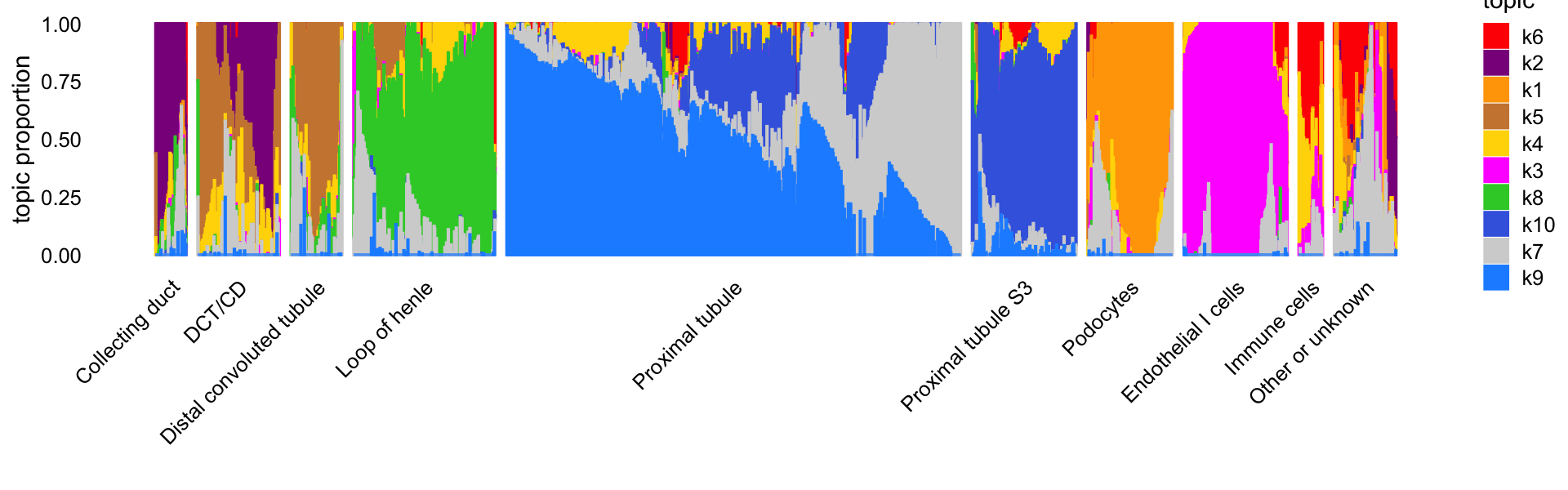
| Version | Author | Date |
|---|---|---|
| 0d6c9fd | Peter Carbonetto | 2022-08-05 |
# grouping
#          Collecting duct                   DCT/CD Distal convoluted tubule
#                      164                      499                      319
#            Loop of henle          Proximal tubule       Proximal tubule S3
#                      814                     2565                      594
#                Podocytes      Endothelial I cells             Immune cells
#                      447                      558                      133
#         Other or unknown
#                      338
Let’s now visualize the topics without the benefit of the previously inferred clusters. Instead, we can use PCs computed from the topic proportions to subdivide the cells into 5 clusters. (Here we are assigning labels to these clusters only to make it easier to refer to them.)
pca <- prcomp(fit$L)$x
pc1 <- pca[,1]
pc2 <- pca[,2]
x <- rep("other",nrow(pca))
x[pc1 < 0] <- "proximal tubule"
x[pc1 > 0 & pc2 > 0.2] <- "endothelial I"
rows <- which(x == "other")
fit2 <- select_loadings(fit,loadings = rows)
pca  <- prcomp(fit2$L)$x
y    <- rep("DCT + CD",nrow(pca))
pc1  <- pca[,1]
pc2  <- pca[,2]
y[pc1 < 0 & pc2 > -0.15] <- "loop of henle"
y[pc1 >= 0 & pc2 > -0.15] <- "podocytes + other"
x[rows] <- y
samples$cluster <- factor(x,c("DCT + CD","loop of henle","proximal tubule",
                              "podocytes + other","endothelial I"))
This is what the Structure plot looks like without any external grouping of the cells:
set.seed(1)
p2 <- structure_plot(fit,grouping = samples$cluster,gap = 20,
                     colors = topic_colors,verbose = FALSE)
table(grouping = samples$cluster)
print(p2)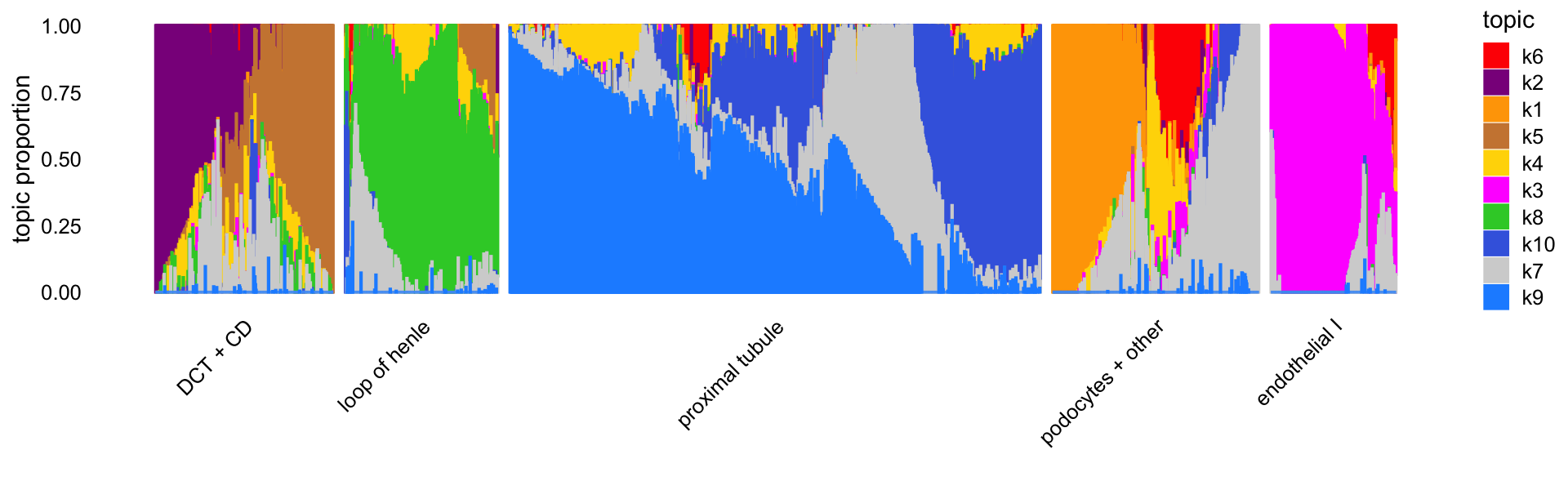
| Version | Author | Date |
|---|---|---|
| 0d6c9fd | Peter Carbonetto | 2022-08-05 |
# grouping
#          DCT + CD     loop of henle   proximal tubule podocytes + other
#              1012               843              2878              1071
#     endothelial I
#               627
The topics clearly identify four distinctive cell types—(1) loop of henle, (2) proximal tubule, (3) distal convoluted tubule (DCT) and collecting duct (CD), and (4) endothelial cells—and within these distinctive cell types there is sometimes a good amount of continuous variation in expression that is further captured by the topics, such as the two topics for DCT and CD, and the heterogeneity among the proximal tubule cells captured by several topics.
Next, let’s see if the gene ranking generated from the differential accessibility analysis of the topics supports these interpretations, and helps us interpret some of the other topics that are less clear such as topic 9.
In this next code chunk we prepare the gene_info and
de_gene data structures for the volcano plots.
data(gene_sets_mouse)
gene_info <- gene_sets_mouse$gene_info
gene_info <- subset(gene_info,!is.na(Ensembl))
gene_info <- subset(gene_info,!duplicated(Ensembl))
ids <- gene_info$Ensembl
ids <- intersect(ids,rownames(de_gene$coef))
de_gene$coef  <- de_gene$coef[ids,]
de_gene$logLR <- de_gene$logLR[ids,]
ids       <- rownames(de_gene$coef)
gene_info <- subset(gene_info,is.element(Ensembl,ids))
rownames(gene_info) <- gene_info$Ensembl
gene_info <- gene_info[ids,]
genes     <- gene_info$Symbol
These next few volcano plots show, for each gene tested for enrichment, the mean LFC on the x-axis against the logBF for enrichment on the y-axis. Marker genes identified in the Park et al paper are highlighted in red.
k <- 2
label_genes <- (is.element(genes,cd_genes) & de_gene$logLR[,k] > 4) |
               (de_gene$logLR[,k] > 35 & de_gene$coef[,k] > 0) |
               (de_gene$coef[,k] > 3)
k2_genes <- genes
k2_genes[!label_genes] <- ""
p2 <- volcano_plot_enrich(de_gene,k = 2,labels = k2_genes,
                          highlight = is.element(genes,cd_genes),
                          ymax = 100)
k <- 5
label_genes <- (is.element(genes,dct_genes) & de_gene$logLR[,k] > 4) |
               (de_gene$logLR[,k] > 40 & de_gene$coef[,k] > 1) |
               (de_gene$coef[,k] > 3)
k5_genes <- genes
k5_genes[!label_genes] <- ""
p5 <- volcano_plot_enrich(de_gene,k = 5,labels = k5_genes,
                          highlight = is.element(genes,dct_genes),
                          ymax = 100)
k <- 3
label_genes <- (is.element(genes,endo_genes) & de_gene$logLR[,k] > 4) |
               (de_gene$logLR[,k] > 85 & de_gene$coef[,k] > 2.25) |
               (de_gene$coef[,k] > 4.5)
k3_genes <- genes
k3_genes[!label_genes] <- ""
p3 <- volcano_plot_enrich(de_gene,k = 3,labels = k3_genes,
                          highlight = is.element(genes,endo_genes),
                          ymax = 125)
k <- 1
label_genes <- (is.element(genes,podo_genes) & de_gene$logLR[,k] > 4) |
               (de_gene$logLR[,k] > 50 & de_gene$coef[,k] > 2) |
               (de_gene$logLR[,k] > 20 & de_gene$coef[,k] > 3.75)
k1_genes <- genes
k1_genes[!label_genes] <- ""
p1 <- volcano_plot_enrich(de_gene,k = 1,labels = k1_genes,
                          highlight = is.element(genes,podo_genes),
                          ymax = 80)
k <- 8
label_genes <- (is.element(genes,loh_genes) & de_gene$logLR[,k] > 4) |
               (de_gene$logLR[,k] > 60 & de_gene$coef[,k] > 0) |
               (de_gene$coef[,k] > 3)
k8_genes <- genes
k8_genes[!label_genes] <- ""
p8 <- volcano_plot_enrich(de_gene,k = 8,labels = k8_genes,
                          highlight = is.element(genes,loh_genes),
                          ymax = 140)
plot_grid(p2,p5,
          p3,p1,
          p8,
          nrow = 3,ncol = 2)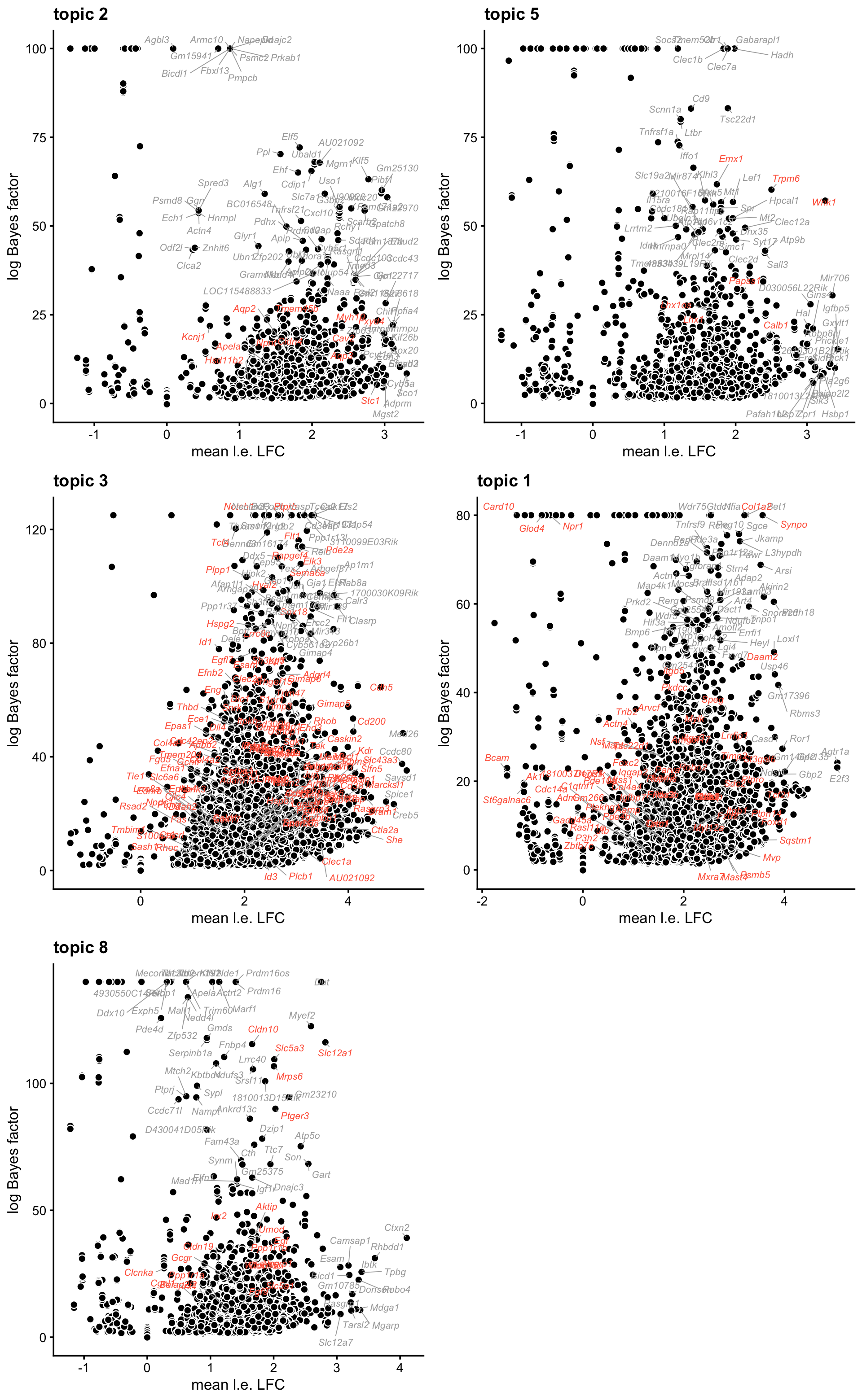
These next two volcano plots also highlight, in blue, the marker genes identified in Wu et al for the S1 and S3 segments of the proximal tubule.
k <- 9
label_genes <- (is.element(genes,S1_genes) &
                de_gene$logLR[,k] > 4) |
               (de_gene$logLR[,k] > 40 & de_gene$coef[,k] > 2.25) |
               (de_gene$logLR[,k] > 100 & de_gene$coef[,k] > 1) |
               (de_gene$coef[,k] > 3)
k9_genes <- genes
k9_genes[!label_genes] <- ""
k9_highlight <- rep(0,length(genes))
k9_highlight[is.element(genes,pt_genes)] <- 1
k9_highlight[is.element(genes,S1_genes)] <- 2
p9 <- volcano_plot_enrich(de_gene,k = 9,labels = k9_genes,
                          highlight = factor(k9_highlight),ymax = 200)
k <- 10
label_genes <- (is.element(genes,S3_genes) &
                de_gene$logLR[,k] > 4) |
               (de_gene$logLR[,k] > 65 & de_gene$coef[,k] > 1.5) |
               (de_gene$coef[,k] > 3)
k10_genes <- genes
k10_genes[!label_genes] <- ""
k10_highlight <- rep(0,length(genes))
k10_highlight[is.element(genes,pt_genes)] <- 1
k10_highlight[is.element(genes,S3_genes)] <- 2
p10 <- volcano_plot_enrich(de_gene,k = 10,labels = k10_genes,
                           highlight = factor(k10_highlight),ymax = 200)
plot_grid(p9,p10,nrow = 1,ncol = 2)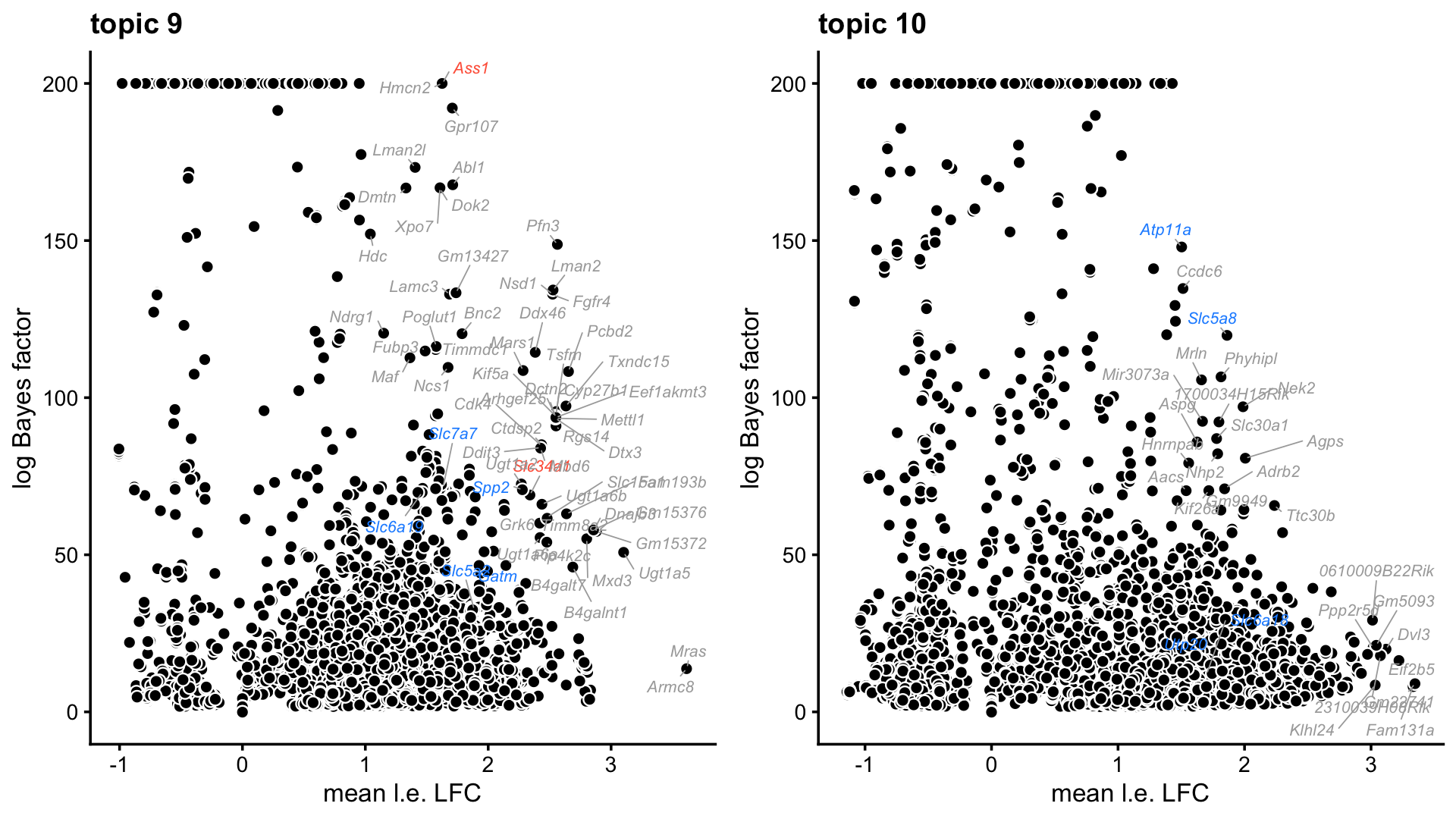
These volcano plots summarize the gene enrichment results for the remaining topics.
To do:
- Create volcano plots for paper. In particular, volcano plots for topics 9 and 10 will go in the main text, and the remaining will go in the supplement. Also, fill out “selected top genes”.
k <- 4
label_genes <- (de_gene$logLR[,k] > 40 & de_gene$coef[,k] > 1.75) |
               (de_gene$logLR[,k] > 10 & de_gene$coef[,k] > 2)
k4_genes <- genes
k4_genes[!label_genes] <- ""
p4 <- volcano_plot_enrich(de_gene,k = 4,labels = k4_genes)
k <- 6
label_genes <- (de_gene$logLR[,k] > 20) |
               (de_gene$logLR[,k] > 10 & de_gene$coef[,k] > 2)
k6_genes <- genes
k6_genes[!label_genes] <- ""
p6 <- volcano_plot_enrich(de_gene,k = 6,labels = k6_genes,ymax = 40)
k <- 7
label_genes <- (de_gene$logLR[,k] > 75 & de_gene$coef[,k] > 0) |
               (de_gene$logLR[,k] > 10 & de_gene$coef[,k] > 1.75) |
               (grepl("Zfp",gene_info$Symbol,fixed = TRUE) &
                de_gene$logLR[,k] > 15)
k7_genes <- genes
k7_genes[!label_genes] <- ""
p7 <- volcano_plot_enrich(de_gene,k = 7,labels = k7_genes,ymax = 200)
plot_grid(p4,p6,p7,nrow = 2,ncol = 2)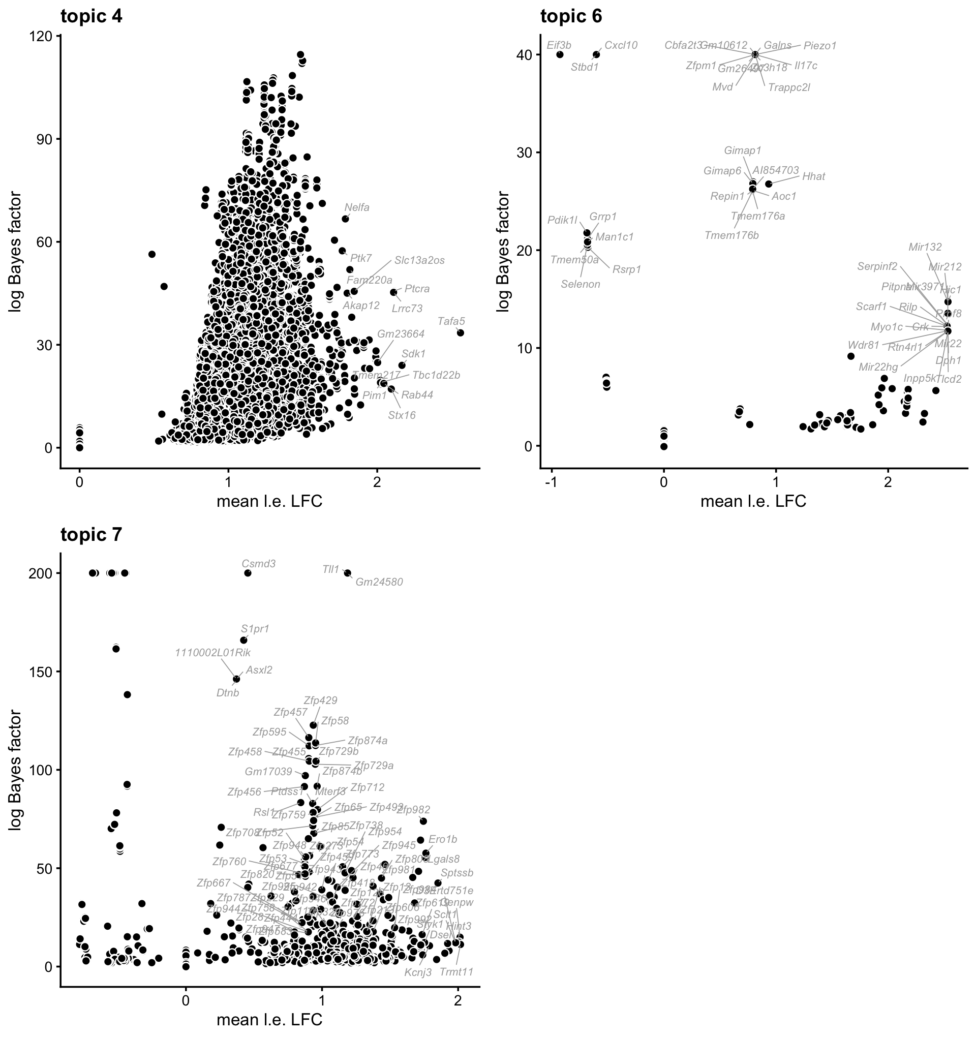
| Version | Author | Date |
|---|---|---|
| b98cc33 | Peter Carbonetto | 2022-10-04 |
Diagram from osmosis.com:
# Warning: Removed 2 rows containing missing values (geom_point).
# Warning: Removed 1 rows containing missing values (geom_point).

# Warning: Removed 1 rows containing missing values (geom_point).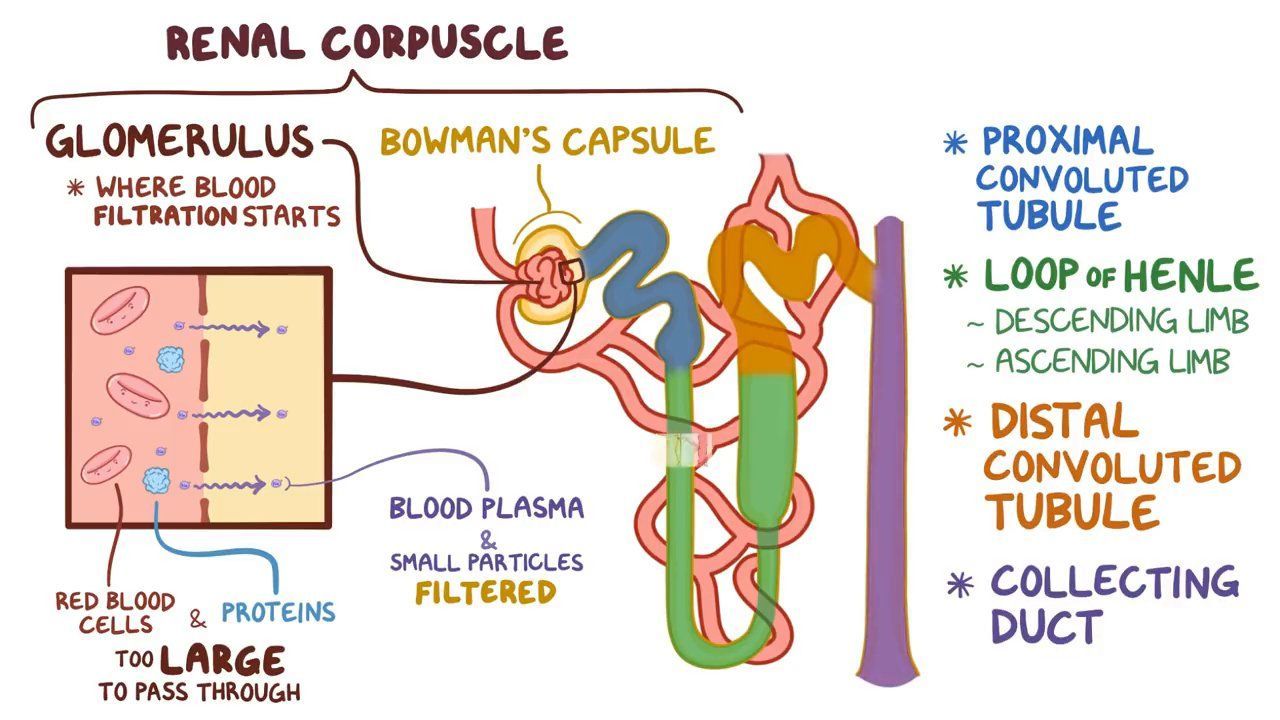
kidney diagram
sessionInfo()
# R version 3.6.2 (2019-12-12)
# Platform: x86_64-apple-darwin15.6.0 (64-bit)
# Running under: macOS Catalina 10.15.7
#
# Matrix products: default
# BLAS:   /Library/Frameworks/R.framework/Versions/3.6/Resources/lib/libRblas.0.dylib
# LAPACK: /Library/Frameworks/R.framework/Versions/3.6/Resources/lib/libRlapack.dylib
#
# locale:
# [1] en_US.UTF-8/en_US.UTF-8/en_US.UTF-8/C/en_US.UTF-8/en_US.UTF-8
#
# attached base packages:
# [1] stats     graphics  grDevices utils     datasets  methods   base
#
# other attached packages:
# [1] cowplot_1.1.1      ggrepel_0.9.1      ggplot2_3.3.6      fastTopics_0.6-131
# [5] pathways_0.1-20    Matrix_1.4-2       workflowr_1.7.0
#
# loaded via a namespace (and not attached):
#  [1] mcmc_0.9-6          fs_1.5.2            progress_1.2.2
#  [4] httr_1.4.2          rprojroot_1.3-2     tools_3.6.2
#  [7] backports_1.1.5     bslib_0.3.1         utf8_1.1.4
# [10] R6_2.4.1            irlba_2.3.3         uwot_0.1.10
# [13] DBI_1.1.0           lazyeval_0.2.2      colorspace_1.4-1
# [16] withr_2.5.0         tidyselect_1.1.1    gridExtra_2.3
# [19] prettyunits_1.1.1   processx_3.5.2      compiler_3.6.2
# [22] git2r_0.29.0        quantreg_5.54       SparseM_1.78
# [25] plotly_4.9.2        labeling_0.3        sass_0.4.0
# [28] scales_1.1.0        SQUAREM_2017.10-1   quadprog_1.5-8
# [31] callr_3.7.0         pbapply_1.5-1       mixsqp_0.3-46
# [34] systemfonts_1.0.2   stringr_1.4.0       digest_0.6.23
# [37] rmarkdown_2.11      MCMCpack_1.4-5      pkgconfig_2.0.3
# [40] htmltools_0.5.2     highr_0.8           fastmap_1.1.0
# [43] invgamma_1.1        htmlwidgets_1.5.1   rlang_0.4.11
# [46] rstudioapi_0.13     farver_2.0.1        jquerylib_0.1.4
# [49] generics_0.0.2      jsonlite_1.7.2      BiocParallel_1.18.1
# [52] dplyr_1.0.7         magrittr_2.0.1      Rcpp_1.0.8
# [55] munsell_0.5.0       fansi_0.4.0         lifecycle_1.0.0
# [58] stringi_1.4.3       whisker_0.4         yaml_2.2.0
# [61] MASS_7.3-51.4       Rtsne_0.15          grid_3.6.2
# [64] parallel_3.6.2      promises_1.1.0      crayon_1.4.1
# [67] lattice_0.20-38     hms_1.1.0           knitr_1.37
# [70] ps_1.6.0            pillar_1.6.2        fgsea_1.15.1
# [73] fastmatch_1.1-0     glue_1.4.2          evaluate_0.14
# [76] getPass_0.2-2       data.table_1.12.8   RcppParallel_5.1.5
# [79] vctrs_0.3.8         httpuv_1.5.2        MatrixModels_0.4-1
# [82] gtable_0.3.0        purrr_0.3.4         tidyr_1.1.3
# [85] assertthat_0.2.1    ashr_2.2-54         xfun_0.29
# [88] coda_0.19-3         later_1.0.0         ragg_0.3.1
# [91] viridisLite_0.3.0   truncnorm_1.0-8     tibble_3.1.3
# [94] ellipsis_0.3.2