Multi-condition differential expression analysis in single-cell RNA-seq data using Poisson mash
Yusha Liu, Peter Carbonetto
2023-11-28
Source:vignettes/intro_poisson_mash.Rmd
intro_poisson_mash.RmdOverview
This vignette illustrates how to use Poisson multivariate adaptive shrinkage (“Poisson mash”) to analyze single-cell RNA-sequencing (scRNA-seq) data. Poisson mash was developed for multi-condition differential expression analysis with scRNA-seq data in which gene expression is measured in many different conditions. The aim is to detect which genes are differentially expressed (DE) and to estimate expression differences (log-fold changes) among multiple conditions. This approach makes use of the multivariate adaptive shrinkage (mash) prior.
We illustrate Poisson mash by analyzing a scRNA-seq data set that was developed in order to learn about the effects of cytokine stimulation on gene expression. We will work through the Poisson mash analysis of this dataa set step-by-step.
First, we load the R packages needed to run the analysis.
We also set the random number generator seed to ensure that the results are reproducible.
set.seed(1)Create a data object for Poisson mash
To run Poisson mash, you need to provide: (1) a matrix of UMI counts, stored as a \(J \times N\) matrix \(Y\) with entries \(y_{ji}\), where \(i = 1, \dots,N\) indexes cells and \(j=1,\dots,J\) indexes genes; and (2) a vector of length \(N\) in which the \(i^{\mathrm{th}}\) element gives the condition label of cell \(i\). We denote the number of conditions by \(R\). (\(R\) should be much larger than 2.)
The original data set contained counts for 13,362 cells, 8,543 genes and 45 conditions (44 cytokine treatments plus one control). For this vignette, we will use subset (1,936 cells, 2,158 genes, 12 conditions), but later we will inspect the results obtained from running Poisson mash on the full data set.
data(neutrophils_subset)
Y <- neutrophils_subset$Y
conditions <- neutrophils_subset$conditions
dim(Y)
conditions <- as.factor(conditions)
table(conditions)
# [1] 2158 1936
# conditions
#    IL10 IL12p70    IL18    IL1a    IL1b     IL2     IL3     IL4     IL5     IL6
#      82     198     254     392     251     109     105     133      81     122
#     IL7     IL9
#     105     104
After loading in the data, we compute the cell-specific size factors. This can be done in various ways. The simplest option is to take the sum of the counts \(y_{ji}\) across all genes in each cell \(i\). Here we take a deconvolution-based approach implemented in scran:
clusters  <- quickCluster(Y)
si        <- calculateSumFactors(Y,clusters = clusters)
names(si) <- colnames(Y)
Next, we create a data object for poisson mash analysis using the
function pois_mash_set_data().
dat <- pois_mash_set_data(Y,conditions,si)By default, Poisson mash assumes a gene-specific baseline expression level, \(\mu_j\), that is shared across all conditions.
(Poisson mash can also handle the more complex setting in which the
\(R\) conditions arise from \(m = 1, \dots, M\) subgroups, and each
subgroup has its own baseline, \(\mu_{jm}\). For example, one may want to
perform a DE analysis across multiple treatment conditions, jointly for
multiple cell types. In this case, \(M\) is the number of cell types, and \(R\) represents the total number of
combinations of treatment conditions and cell types. Please refer to the
documentation for the function pois_mash_set_data() to see
how to do this.)
Estimate latent factors capturing unwanted variation
Unwanted variation present in the data can induce dependence among gene-wise tests and confound the DE analysis. In some cases, the confounding variables are known, such as when these capture batch effects. More often, the unwanted variation is due to unmeasured factors. Here we estimate the unmeasured confounding variables using glmpca.
design <- model.matrix(~conditions)
fit.glmpca <- glmpca(Y = as.matrix(Y),X = design[,-1],L  = 4,fam = "nb2",
                     sz = si,ctl = list(minIter = 1,maxIter = 20,
                                        verbose = TRUE))
Fuv <- as.matrix(fit.glmpca$loadings)
For this vignette, we ran glmpca for only 20 iterations,
but typically it is better to perform more iterations (100, or perhaps
more).
Fit the Poisson mash model
Step 1: Prefit the model
We first fit Poisson mash under the assumption of no DE to get sensible initial estimates of the other model parameters, including the gene-specific baseline expressions \(\mu_j\). (See the paper for details.)
prefit <- pois_mash_prefit(dat,ruv = TRUE,Fuv = Fuv,verbose = TRUE)Step 2: Set up the prior covariance matrices
Let the \(R \times 1\) vector \(\beta_j = (\beta_{j1}, \dots, \beta_{jR})'\) denote the true DE effects of each of the \(R\) conditions relative to the baseline expression \(\mu_j\) for gene \(j\). We assume that \(\beta_j\) follows a “mash prior”, which is a mixture of multivariate normal distributions: \[ p(\beta_j; \pi, U) = \sum_{k=1}^K \sum_{l=1}^L \pi_{kl} N_R(\beta_j; 0, w_l U_k). \] In the mash prior, \(w_l\) is a pre-specified grid of scaling coefficients, spanning from very small to very large to capture the full range of possible DE effect sizes; each \(U_k\) is a covariance matrix that captures a different pattern of covariation across conditions; \(\pi_{kl}\) are the mixture proportions that are estimated from the data during model fitting.
To use Poisson mash, you need to specify these prior covariance matrices. This may include “canonical” covariance matrices that represent, for example, DE specific to a condition; and “data-driven” covariance matrices that are learned from the data and can capture arbitrary patterns of DE among conditions.
For the canonical matrices, here we consider the matrices capturing
condition-specific effects for each of the \(R\) conditions. These matrices can be
generated using the pois_cov_canonical() function:
ulist.c <- pois_cov_canonical(dat)Data-driven covariance matrices are estimated using a three-step
process: (1) initialization, (2) refinement, (3) diagonal entry
modification. The initialization phase is implemented by the function
pois_cov_init(). To estimate the data-driven covariance
matrices, we only use the subset of genes containing “strong signals”;
that is, the genes that are considered DE by a multinomial
goodness-of-fit test. The selection of genes with strong signals is
implicitly performed by the call to pois_cov_init(), e.g.,
setting cutoff = 3 selects the genes for which the
magnitude of z-score (inverted from the p-value of the goodness-of-fit
test) exceeds 3.
res.pca <- pois_cov_init(dat,cutoff = 3)The refinement phase refines the initial estimates of data-driven
covariance matrices using the Extreme Deconvolution (ED) algorithm, and
is implemented by the function pois_cov_ed(). As in the
initialization phase, only data from the genes with strong signals are
used. It should be noted that only the data-driven covariance matrices
need to be refined, so they need to be distinguished from the canonical
covariance matrices in the pois_cov_ed() call using the
argument ulist.dd.
R <- ncol(dat$X)
# Merge data-driven and canonical rank-1 prior covariance matrices.
ulist <- c(res.pca$ulist,ulist.c)
# Specify whether a rank-1 prior covariance matrix is data-driven
# or not (note all full-rank covariance matrices are data-driven
# so do not need this specification).
ulist.dd <- c(rep(TRUE,length(res.pca$ulist) - 1),rep(FALSE,R + 1))
# Run ED on the genes with strong signals.
fit.ed <- pois_cov_ed(dat,subset = res.pca$subset,Ulist = res.pca$Ulist,
                      ulist = ulist,ulist.dd = ulist.dd,ruv = TRUE,
                      Fuv = Fuv,verbose = TRUE,init = prefit,
                      control = list(maxiter = 10))
For the purposes of this vignette, we just ran
pois_cov_ed() for 10 iterations, but we recommend
performing more iterations when analyzing your own data (the default
number of iterations is 500).
The modification phase adds a small constant \(\epsilon^2\) (e.g., 0.01) to the diagonal entries of the estimated data-driven covariance matrices. This step is done to alleviate issues of inflated local false sign rates (lfsr) (the lfsr is analogous to but typically more more conservative than a local false discovery rate).
# Add epsilon2*I to each full-rank data-driven prior covariance matrix.
Ulist <- fit.ed$Ulist
H <- length(Ulist)
for(h in 1:H){
  Uh <- Ulist[[h]]
  Uh <- Uh/max(diag(Uh))
  Ulist[[h]] <- Uh + 0.01*diag(R)
}

# Add epsilon2*I to each rank-1 data-driven prior covariance matrix.
G <- length(fit.ed$ulist)
epsilon2.G <- rep(1e-8,G)
names(epsilon2.G) <- names(fit.ed$ulist)
epsilon2.G[ulist.dd] <- 0.01
Step 3: Fit the Poisson mash model
Now we are ready to fit the Poisson mash model to data from all
genes, which is implemented by the function
pois_mash().
By default, differences in expression are measured relative to the
mean across all conditions. (To change how expression differences are
measured, see the pois_mash() input arguments
C and res.colnames. See also the
median_deviations input argument for computing differences
relative to medians as well as means.)
res <- pois_mash(data = dat,Ulist = Ulist,ulist = fit.ed$ulist,
                 ulist.epsilon2 = epsilon2.G,gridmult = 2.5,ruv = TRUE,
                 Fuv = Fuv,rho = prefit$rho,verbose = TRUE,
                 init = list(mu = prefit$mu,psi2 = prefit$psi2),
                 control = list(maxiter = 10,nc = 2))
For this vignette, we ran pois_mash() for only 10
iterations, but in practice we recommend setting
maxiter = 100, or perhaps more.
Examining the Poisson mash results
Above, we illustrated the steps involved in analyzing scRNA-seq data using Poisson mash. Separately, we analyzed the full scRNA-seq data set using this script, and here we examine the results of this analysis on the full data.
data(neutrophils_pois_mash_ruv_fit)The Poisson mash result provides posterior summaries of the condition-specific DE effects relative to the reference condition, including: posterior means and posterior standard deviations of the log-fold changes (LFCs); and measures of significance for the LFCs (local false sign rates). These posterior quantities are stored in the “result” output. For example, this gives the posterior mean estimates of the LFCs:
head(neutrophils_pois_mash_ruv_fit$result$PosteriorMean)/log(2)
#                Ctrl_2-mean    CCL20-mean    CXCL1-mean    CCL22-mean
# Mrpl15        -0.034042592 -0.0074681827  0.0104375255 -0.0212980437
# Lypla1        -0.009057545 -0.0028162390 -0.0312773830 -0.0100671020
# Tcea1          0.006406279  0.0031637077  0.0117792404  0.0112956807
# Atp6v1h        0.005641873  0.0043244408 -0.0009984417  0.0001755186
# Rb1cc1         0.005531303  0.0105905421 -0.0071790326  0.0060939489
# 4732440D04Rik -0.008846585 -0.0003553177  0.0248291673 -0.0009278163
#                 CXCL5-mean   CCL11-mean     CCL4-mean    CCL17-mean
# Mrpl15        -0.017696220 -0.005062400 -0.0188073088 -0.0004958562
# Lypla1        -0.011641034 -0.034870283 -0.0052598409 -0.0489983029
# Tcea1          0.007417445  0.018070010  0.0059066159  0.0251398080
# Atp6v1h        0.002388297 -0.002812183  0.0002977357 -0.0038973739
# Rb1cc1         0.003342450 -0.011461863  0.0064281778 -0.0279408869
# 4732440D04Rik -0.003123874  0.025364909 -0.0059579239  0.0390409658
#                  CCL5-mean   CXCL13-mean  CXCL10-mean   CXCL9-mean  CXCL12-mean
# Mrpl15        -0.033427164 -0.0193033143 -0.030417476 -0.022281407 -0.025163326
# Lypla1        -0.007691913 -0.0085652232 -0.011486987 -0.014891750 -0.008054578
# Tcea1          0.004426990  0.0103737032  0.013105638  0.017414325  0.006215443
# Atp6v1h        0.003540437  0.0084019881  0.004709271  0.001339506  0.001860474
# Rb1cc1         0.006098348  0.0154390774  0.014276063  0.006610999  0.002812130
# 4732440D04Rik -0.009417124 -0.0001110654 -0.004154084  0.005365928 -0.002993656
#                 GCSF-mean    MCSF-mean    GMCSF-mean    IFNg-mean    IL10-mean
# Mrpl15        -0.04762754 -0.011974981 -0.0040743996  0.073542495 -0.019084842
# Lypla1         0.14384314 -0.003109597 -0.0081087780 -0.039236940 -0.007648764
# Tcea1         -0.05427278  0.001577959  0.0023373278  0.003621784  0.003729513
# Atp6v1h       -0.02877024  0.003926684 -0.0009182916  0.019606260  0.002691518
# Rb1cc1         0.03195692  0.003707192 -0.0001500394 -0.029808303 -0.002084963
# 4732440D04Rik -0.06384574 -0.007555636 -0.0007171226  0.023251851 -0.009499298
#                IL12p70-mean   IL17a-mean    IL13-mean    IL15-mean
# Mrpl15         0.2576041103 -0.001024305  0.011740475  0.035485679
# Lypla1        -0.0828283220 -0.046523655 -0.009346285 -0.025208920
# Tcea1         -0.0009465631  0.018992787  0.005639251 -0.002893936
# Atp6v1h        0.0342083395 -0.001067275 -0.008369830  0.011317109
# Rb1cc1        -0.1651456352 -0.018245683 -0.009315472 -0.012970846
# 4732440D04Rik  0.1364570899  0.026939736  0.021427294  0.012409178
#                  IL17f-mean    IL22-mean   IL18-mean   IL1a-mean     IL2-mean
# Mrpl15        -0.0214237310 -0.027338931  0.13505580  0.17858759 -0.011638392
# Lypla1        -0.0262238707 -0.025832683 -0.09694090  0.37605931 -0.013308553
# Tcea1          0.0160574340  0.018964004  0.01279576 -0.16013889  0.005249033
# Atp6v1h        0.0051885570  0.009948429  0.04888996 -0.13480913  0.007314477
# Rb1cc1        -0.0029898176  0.004610991 -0.06709438  0.09961320  0.001127090
# 4732440D04Rik  0.0001264711 -0.006596828  0.05459626 -0.07111402 -0.008259135
#                    IL3-mean   IL1b-mean    IL23-mean    IL21-mean    IL33-mean
# Mrpl15        -0.0009068703  0.05281386 -0.042690753 -0.034675571  0.018658887
# Lypla1        -0.0082352512  0.31148869 -0.004993754 -0.020986050 -0.034343159
# Tcea1          0.0041293566 -0.13669710  0.008776216  0.010878092  0.011885645
# Atp6v1h        0.0044677986 -0.06724345  0.003236710  0.006627147  0.012358900
# Rb1cc1         0.0056172066  0.07400191  0.007084813  0.005422794 -0.013401797
# 4732440D04Rik  0.0023447159 -0.11975825 -0.004488205 -0.001061083  0.006579908
#                  IL25-mean     IL34-mean   IL36a-mean     IL4-mean     IL6-mean
# Mrpl15        -0.016490274 -0.0164906818 -0.002782744 -0.027822774 -0.030788378
# Lypla1        -0.017875933  0.0008588503 -0.005382598 -0.011071839 -0.014087099
# Tcea1          0.008257777 -0.0021607365  0.002050769  0.008573827  0.008767113
# Atp6v1h        0.001986599 -0.0023217803  0.005815554  0.003513273  0.006532946
# Rb1cc1        -0.003602535  0.0068418637 -0.000534509  0.017830621  0.008586397
# 4732440D04Rik -0.002212745 -0.0133139487 -0.005107259 -0.004839267 -0.005515926
#                   IL5-mean      IL7-mean     IL9-mean    IL11-mean    TGFb-mean
# Mrpl15        -0.022185494 -0.0158299311 -0.023641709 -0.025434091 -0.050005560
# Lypla1        -0.007578267 -0.0099514961 -0.013130808 -0.007497674 -0.011780427
# Tcea1          0.004431804  0.0059533811  0.006840927  0.001427087  0.006641472
# Atp6v1h        0.002658004  0.0003339911  0.008573222  0.005973927  0.003977395
# Rb1cc1         0.011690195  0.0080848387  0.001159327  0.005354917  0.008766968
# 4732440D04Rik -0.002355840 -0.0039932668  0.002081985 -0.008332532 -0.010743094
#                  CCL2-mean     CCL3-mean    TSLP-mean
# Mrpl15        -0.034567597 -0.0103474167 -0.039616166
# Lypla1        -0.027622491 -0.0352499237 -0.013467768
# Tcea1          0.012298922  0.0173536034  0.009164278
# Atp6v1h        0.006248766 -0.0006421229  0.003775009
# Rb1cc1         0.010470586 -0.0140145528 -0.003210554
# 4732440D04Rik -0.003063816  0.0176087841 -0.010163785
Here, we divided by log(2) to obtain LFC estimates using
the base-2 logarithm, which is the convention in differential expression
analyses. (The LFCs returned by pois_mash() are on the
natural log-scale.)
These are the local false sign rates (lfsrs) corresponding to these LFC estimates:
head(neutrophils_pois_mash_ruv_fit$result$lfsr)
#               Ctrl_2-mean CCL20-mean CXCL1-mean CCL22-mean CXCL5-mean
# Mrpl15          0.2527081  0.4012463  0.4501408  0.3236194  0.3458751
# Lypla1          0.4041496  0.4586630  0.2824110  0.3962331  0.3803850
# Tcea1           0.4273815  0.4727043  0.3991172  0.3839887  0.4144509
# Atp6v1h         0.4512667  0.4597141  0.4917574  0.4894398  0.4710016
# Rb1cc1          0.4402427  0.3958559  0.4170690  0.4337283  0.4628668
# 4732440D04Rik   0.4327946  0.4654769  0.3436250  0.4950268  0.4815622
#               CCL11-mean CCL4-mean CCL17-mean CCL5-mean CXCL13-mean CXCL10-mean
# Mrpl15         0.4503198 0.3341797  0.4890418 0.2597855   0.3272724   0.2708464
# Lypla1         0.2825026 0.4510857  0.2562523 0.4106041   0.3939088   0.3778143
# Tcea1          0.3573428 0.4453036  0.3363813 0.4379274   0.3983058   0.3799305
# Atp6v1h        0.4959188 0.4908357  0.4919694 0.4657350   0.4275249   0.4526731
# Rb1cc1         0.3991688 0.4255101  0.3040819 0.4316898   0.3563062   0.3636811
# 4732440D04Rik  0.3422911 0.4339455  0.2909048 0.4412258   0.4881681   0.4554252
#               CXCL9-mean CXCL12-mean GCSF-mean MCSF-mean GMCSF-mean IFNg-mean
# Mrpl15         0.3140237   0.2992497 0.3862640 0.3833967  0.4622146 0.2401656
# Lypla1         0.3614019   0.4142332 0.1452817 0.4530279  0.4303208 0.3312796
# Tcea1          0.3414202   0.4310399 0.3113968 0.4735670  0.4699903 0.4753059
# Atp6v1h        0.4792271   0.4775559 0.4042329 0.4627960  0.4971617 0.4117819
# Rb1cc1         0.4318283   0.4606759 0.3334752 0.4614786  0.4997896 0.2825765
# 4732440D04Rik  0.4638220   0.4692696 0.2762227 0.4438452  0.5003250 0.3659072
#               IL10-mean IL12p70-mean IL17a-mean IL13-mean IL15-mean IL17f-mean
# Mrpl15        0.3427273    0.1744947  0.4716441 0.4123012 0.3177474  0.3106887
# Lypla1        0.4247063    0.3924265  0.2288754 0.4595318 0.3401948  0.2803512
# Tcea1         0.4475322    0.4999636  0.3517753 0.4708802 0.4989087  0.3444343
# Atp6v1h       0.4742497    0.4494211  0.4919772 0.4406686 0.4237398  0.4452778
# Rb1cc1        0.4896823    0.1491159  0.3438041 0.4111042 0.3677096  0.4624288
# 4732440D04Rik 0.4375540    0.2703745  0.3192068 0.3842615 0.3906055  0.4873929
#               IL22-mean IL18-mean  IL1a-mean  IL2-mean  IL3-mean  IL1b-mean
# Mrpl15        0.2840685 0.2496381 0.24094477 0.3844175 0.4771050 0.38724729
# Lypla1        0.2920991 0.2921420 0.08710416 0.3715688 0.4046607 0.07767338
# Tcea1         0.3285671 0.4618855 0.23738905 0.4318351 0.4480975 0.22084556
# Atp6v1h       0.4171052 0.3896886 0.32148386 0.4329320 0.4559605 0.37399802
# Rb1cc1        0.4562436 0.2469379 0.22706304 0.4864023 0.4489441 0.24520985
# 4732440D04Rik 0.4636854 0.3521125 0.33522628 0.4499985 0.4692893 0.21622228
#               IL23-mean IL21-mean IL33-mean IL25-mean IL34-mean IL36a-mean
# Mrpl15        0.2345988 0.2530787 0.3984001 0.3534076 0.3745368  0.4676462
# Lypla1        0.4452661 0.3332269 0.2552843 0.3322697 0.4987002  0.4289364
# Tcea1         0.4187680 0.3950206 0.3904403 0.4001663 0.4996069  0.4686664
# Atp6v1h       0.4749808 0.4440192 0.4012765 0.4721274 0.4913212  0.4443712
# Rb1cc1        0.4226749 0.4423292 0.3448722 0.4573188 0.4255365  0.4920261
# 4732440D04Rik 0.4573653 0.4841981 0.4080683 0.4918012 0.4243858  0.4715751
#                IL4-mean  IL6-mean  IL5-mean  IL7-mean  IL9-mean IL11-mean
# Mrpl15        0.2829187 0.2736145 0.3188849 0.3494112 0.3107035 0.3113687
# Lypla1        0.3931525 0.3754091 0.4300739 0.3971178 0.3768724 0.4279538
# Tcea1         0.4204489 0.4090162 0.4498226 0.4286115 0.4221452 0.4548560
# Atp6v1h       0.4638306 0.4447204 0.4752750 0.4886532 0.4290461 0.4639057
# Rb1cc1        0.3258085 0.4049600 0.3723182 0.4111479 0.4849725 0.4372864
# 4732440D04Rik 0.4380127 0.4538717 0.4691893 0.4712914 0.4881865 0.4532162
#               TGFb-mean CCL2-mean CCL3-mean TSLP-mean
# Mrpl15        0.2069668 0.2603012 0.4277883 0.2431181
# Lypla1        0.4058294 0.2903189 0.2679369 0.3818475
# Tcea1         0.4355067 0.3798035 0.3524328 0.4064448
# Atp6v1h       0.4692016 0.4438632 0.4932315 0.4665161
# Rb1cc1        0.4064475 0.4005704 0.3684423 0.4793225
# 4732440D04Rik 0.4158820 0.4869377 0.3579516 0.4369963
We can find the number of differentially expressed genes, which are defined as genes having lfsr less than \(\alpha\) in at least one condition, where \(\alpha\) is a threshold specified by the user (e.g., 0.05):
lfsr <- neutrophils_pois_mash_ruv_fit$result$lfsr
min.lfsr <- apply(lfsr,1,min)
sum(min.lfsr < 0.05)
# [1] 2636
The estimates of other model parameters are stored in the
pois.mash.fit component. For example, the mixture
proportions \(\pi_{kl}\) for
combinations of different scaling coefficients \(w_l\) and prior covariance matrices \(U_k\) tell us which sharing patterns were
estimated to be most prominent in the data:
pheatmap(neutrophils_pois_mash_ruv_fit$pois.mash.fit$pi,
         cluster_rows = FALSE,cluster_cols = FALSE,fontsize_row = 6,
         fontsize_col = 6,main = "")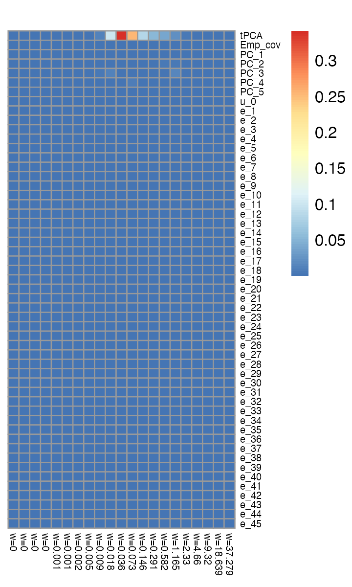
The “tPCA” covariance matrix has by far the largest mixture weight (91% when summed over all scalings, i.e., over columns in this plot). This is the correlation matrix obtained from this covariance matrix (shown here for 27 of the 45 conditions):
data(condition_colors)
U <- neutrophils_pois_mash_ruv_fit$pois.mash.fit$Ulist$tPCA
colnames(U) <- colnames(neutrophils_pois_mash_ruv_fit$pois.mash.fit$mu)
rownames(U) <- colnames(neutrophils_pois_mash_ruv_fit$pois.mash.fit$mu)
idx.trts <- match(names(condition_colors),
                  colnames(neutrophils_pois_mash_ruv_fit$pois.mash.fit$mu))
corr <- cov2cor(U[idx.trts,idx.trts])
pheatmap(corr,cluster_rows = FALSE,cluster_cols = FALSE,angle_col = 90,
         fontsize = 7,main = "")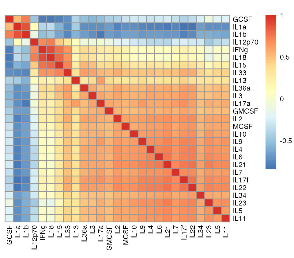
This correlation matrix suggests strong sharing of DE effects among two groups of cytokines: (1) IL-1\(\alpha\), IL-1\(\beta\), G-CSF and (2) IL-12 p70, IFN-\(\gamma\), IL-18, IL-15, IL-33.
Here’s a few differentially expressed genes that show effect sharing among the first group of cytokines:
cols <- colorRampPalette(c("blue","white","red"))(99)
brks <- seq(-log2(10),log2(10),length = 100)
genes1 <- c("Prok2","Nos2","Teddm3","Lipg","Saa3","Wfdc17","Cd38","Ggt1",
            "Dpep2","Mmp19")
pdat <- t(neutrophils_pois_mash_ruv_fit$result$PosteriorMean[genes1,idx.trts])/log(2)
pheatmap(pdat,cluster_rows = FALSE,cluster_cols = FALSE,color = cols,
         breaks = brks,angle_col = 90,fontsize = 7,main = "")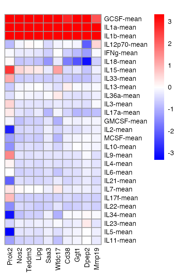
These genes show strong effect sharing among the second group of cytokines:
genes2 <- c("Gbp2","Gbp3","Gbp4","Gbp5","Ifi47","Ifit2","Ifit3","Socs1",
            "Tgtp2","Zbp1")
pdat <- t(neutrophils_pois_mash_ruv_fit$result$PosteriorMean[genes2, idx.trts])/log(2)
pheatmap(pdat,cluster_rows = FALSE,cluster_cols = FALSE,color = cols,
         breaks = brks,angle_col = 90,fontsize = 7,main = "")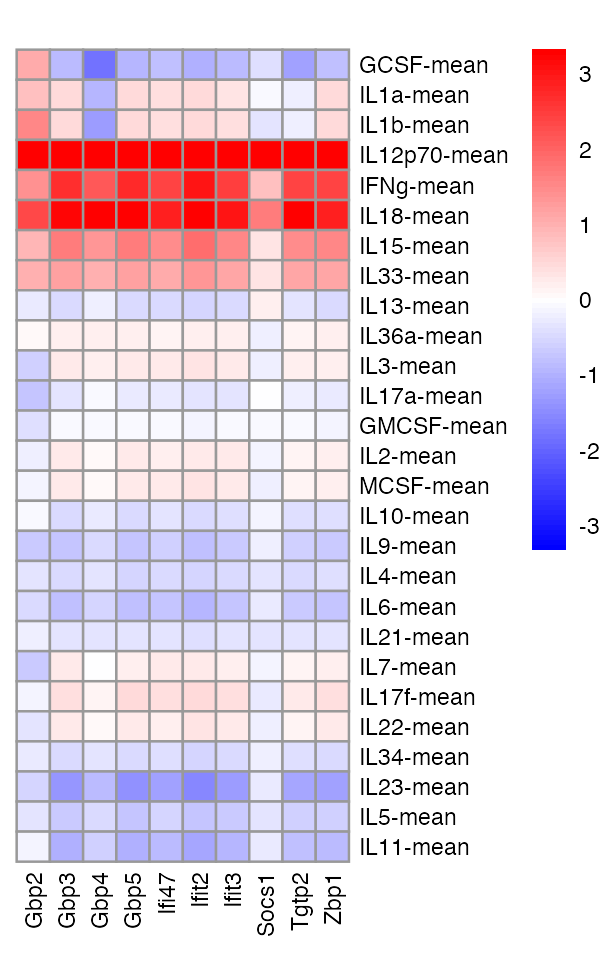
Session info
This is the version of R and the packages that were used to generate these results:
sessionInfo()
# R version 3.6.2 (2019-12-12)
# Platform: x86_64-apple-darwin15.6.0 (64-bit)
# Running under: macOS Catalina 10.15.7
#
# Matrix products: default
# BLAS:   /Library/Frameworks/R.framework/Versions/3.6/Resources/lib/libRblas.0.dylib
# LAPACK: /Library/Frameworks/R.framework/Versions/3.6/Resources/lib/libRlapack.dylib
#
# locale:
# [1] en_US.UTF-8/en_US.UTF-8/en_US.UTF-8/C/en_US.UTF-8/en_US.UTF-8
#
# attached base packages:
# [1] parallel  stats4    stats     graphics  grDevices utils     datasets
# [8] methods   base
#
# other attached packages:
#  [1] poisson.mash.alpha_0.1-98   pheatmap_1.0.12
#  [3] glmpca_0.2.0                scran_1.14.6
#  [5] SingleCellExperiment_1.8.0  SummarizedExperiment_1.16.1
#  [7] DelayedArray_0.12.3         BiocParallel_1.18.1
#  [9] matrixStats_0.63.0          Biobase_2.46.0
# [11] GenomicRanges_1.38.0        GenomeInfoDb_1.22.1
# [13] IRanges_2.20.2              S4Vectors_0.24.4
# [15] BiocGenerics_0.32.0         Matrix_1.3-4
#
# loaded via a namespace (and not attached):
#  [1] bitops_1.0-6             fs_1.5.2                 RColorBrewer_1.1-2
#  [4] rprojroot_2.0.3          tools_3.6.2              bslib_0.3.1
#  [7] utf8_1.1.4               R6_2.4.1                 irlba_2.3.3
# [10] vipor_0.4.5              DBI_1.1.0                colorspace_1.4-1
# [13] tidyselect_1.1.1         gridExtra_2.3            compiler_3.6.2
# [16] cli_3.5.0                BiocNeighbors_1.2.0      desc_1.2.0
# [19] sass_0.4.0               scales_1.1.0             mvtnorm_1.0-11
# [22] SQUAREM_2017.10-1        mixsqp_0.3-48            pkgdown_2.0.7
# [25] systemfonts_1.0.2        stringr_1.4.0            digest_0.6.23
# [28] rmarkdown_2.21           XVector_0.26.0           scater_1.14.6
# [31] pkgconfig_2.0.3          htmltools_0.5.4          highr_0.8
# [34] invgamma_1.1             fastmap_1.1.0            limma_3.42.2
# [37] rlang_1.0.6              DelayedMatrixStats_1.6.1 jquerylib_0.1.4
# [40] generics_0.0.2           jsonlite_1.7.2           dplyr_1.0.7
# [43] RCurl_1.98-1.2           magrittr_2.0.1           BiocSingular_1.2.2
# [46] GenomeInfoDbData_1.2.2   Rcpp_1.0.8               ggbeeswarm_0.6.0
# [49] munsell_0.5.0            fansi_0.4.0              abind_1.4-5
# [52] viridis_0.5.1            lifecycle_1.0.3          stringi_1.4.3
# [55] yaml_2.2.0               edgeR_3.28.1             MASS_7.3-51.4
# [58] zlibbioc_1.32.0          grid_3.6.2               dqrng_0.2.1
# [61] crayon_1.4.1             lattice_0.20-38          locfit_1.5-9.4
# [64] knitr_1.37               pillar_1.6.2             igraph_1.2.5
# [67] glue_1.4.2               evaluate_0.14            vctrs_0.3.8
# [70] gtable_0.3.0             purrr_0.3.4              assertthat_0.2.1
# [73] ashr_2.2-57              ggplot2_3.3.6            xfun_0.36
# [76] rsvd_1.0.2               ragg_0.3.1               viridisLite_0.3.0
# [79] truncnorm_1.0-8          tibble_3.1.3             poilog_0.4
# [82] beeswarm_0.2.3           memoise_1.1.0            seqgendiff_1.2.2
# [85] statmod_1.4.34           ellipsis_0.3.2