Apply mash method to data

Apply mash method to data

mash(
  data,
  Ulist = NULL,
  gridmult = sqrt(2),
  grid = NULL,
  normalizeU = TRUE,
  usepointmass = TRUE,
  g = NULL,
  fixg = FALSE,
  prior = c("nullbiased", "uniform"),
  nullweight = 10,
  optmethod = c("mixSQP", "mixIP", "mixEM", "cxxMixSquarem"),
  control = list(),
  verbose = TRUE,
  add.mem.profile = FALSE,
  algorithm.version = c("Rcpp", "R"),
  pi_thresh = 1e-10,
  A = NULL,
  posterior_samples = 0,
  seed = 123,
  outputlevel = 2,
  output_lfdr = FALSE
)

Arguments

data

a mash data object containing the Bhat matrix, standard errors, alpha value; created using mash_set_data or mash_set_data_contrast

Ulist

a list of covariance matrices to use (see normalizeU for rescaling these matrices)

gridmult

scalar indicating factor by which adjacent grid values should differ; close to 1 for fine grid

grid

vector of grid values to use (scaling factors omega in paper)

normalizeU

whether or not to normalize the U covariances to have maximum of 1 on diagonal

usepointmass

whether to include a point mass at 0, corresponding to null in every condition

g

the value of g obtained from a previous mash fit - an alternative to supplying Ulist, grid and usepointmass

fixg

if g is supplied, allows the mixture proportions to be fixed rather than estimated; e.g., useful for fitting mash to test data after fitting it to training data

prior

indicates what penalty to use on the likelihood, if any

nullweight

scalar, the weight put on the prior under “nullbiased” specification, see “prior”.

optmethod

name of optimization method to use

control

A list of control parameters passed to optmethod.

verbose

If TRUE, print progress to R console.

add.mem.profile

If TRUE, print memory usage to R console (requires R library `profmem`).

algorithm.version

Indicates whether to use R or Rcpp version

pi_thresh

threshold below which mixture components are ignored in computing posterior summaries (to speed calculations by ignoring negligible components)

A

the linear transformation matrix, Q x R matrix. This is used to compute the posterior for Ab.

posterior_samples

the number of samples to be drawn from the posterior distribution of each effect.

seed

A random number seed to use when sampling from the posteriors. It is used when posterior_samples > 0.

outputlevel

controls amount of computation / output; 1: output only estimated mixture component proportions, 2: and posterior estimates, 3: and posterior covariance matrices, 4: and likelihood matrices

output_lfdr

If output_lfdr = TRUE, output local false discovery rate estimates. The lfdr tends to be sensitive to mis-estimated covariance matrices, and generally we do not recommend using them; we recommend using the local false sign rate (lfsr) instead, which is always returned, even when output_lfdr = TRUE.

Value

a list with elements result, loglik and fitted_g

Examples

Bhat     = matrix(rnorm(100),ncol=5) # create some simulated data
Shat     = matrix(rep(1,100),ncol=5)
data     = mash_set_data(Bhat,Shat, alpha=1)
U.c      = cov_canonical(data)
res.mash = mash(data,U.c)
#>  - Computing 20 x 121 likelihood matrix.
#>  - Likelihood calculations took 0.00 seconds.
#>  - Fitting model with 121 mixture components.
#>  - Model fitting took 0.05 seconds.
#>  - Computing posterior matrices.
#>  - Computation allocated took 0.00 seconds.

# Run mash with penalty exponent on null term equal to 100.
# See "False disovery rates: a new deal" (M. Stephens 2017),
# supplementary material S.2.5 for more details.
set.seed(1)
simdata = simple_sims(500,5,1)
data    = mash_set_data(simdata$Bhat,simdata$Shat)
U.c     = cov_canonical(data)
res0    = mash(data,U.c)
#>  - Computing 2000 x 151 likelihood matrix.
#>  - Likelihood calculations took 0.05 seconds.
#>  - Fitting model with 151 mixture components.
#>  - Model fitting took 0.57 seconds.
#>  - Computing posterior matrices.
#>  - Computation allocated took 0.01 seconds.
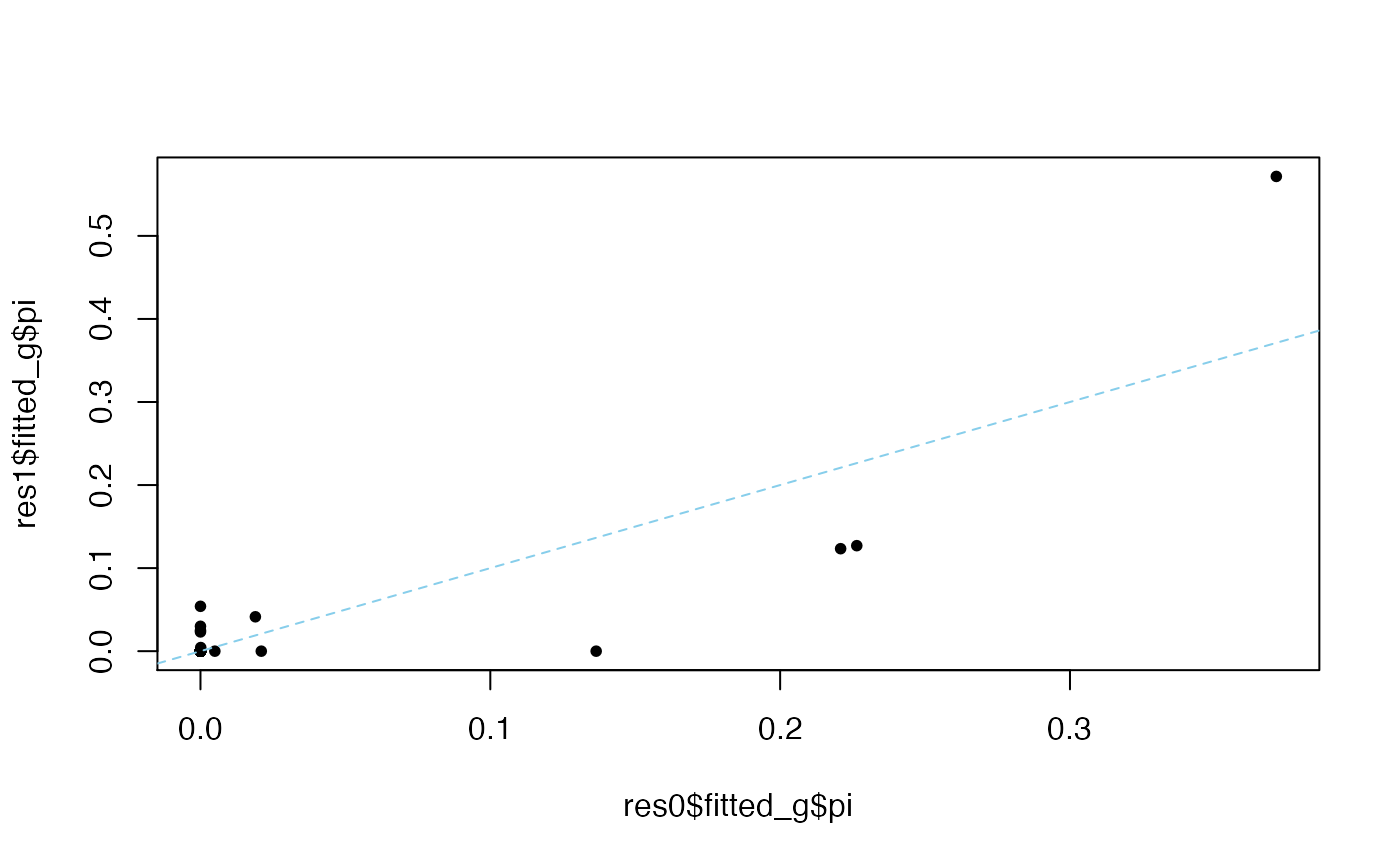
res1    = mash(data,U.c,prior = "nullbiased",nullweight = 101)
#>  - Computing 2000 x 151 likelihood matrix.
#>  - Likelihood calculations took 0.04 seconds.
#>  - Fitting model with 151 mixture components.
#>  - Model fitting took 0.54 seconds.
#>  - Computing posterior matrices.
#>  - Computation allocated took 0.02 seconds.
plot(res0$fitted_g$pi,res1$fitted_g$pi,pch = 20)
abline(a = 0,b = 1,col = "skyblue",lty = "dashed")