Accounting for covariates in fSuSiE
William R.P. Denault
2026-05-13
Source:vignettes/Adjusting_covariate.Rmd
Adjusting_covariate.RmdAdjustment for functional fine-mapping
In order to reduce the number of false positives in fine-mapping analysis, it is often important to account for potential confounders. As most of the tools in the SuSiE suite don’t account for confounders while performing fine-mapping, it is important to account for confounders prior to the analysis. A similar problem arises with fSuSiE. While it is relatively straightforward to adjust univariate phenotypes. It is more complicated to adjust curves/profiles for confounding. Thus, we implemented a user-friendly function that performs this preprocessing step.
Generating the data
knitr::opts_chunk$set(
    echo = TRUE,
    message = FALSE,
    warning = FALSE
)
library(fsusieR)
library(susieR)
#>
#> Attaching package: 'susieR'
#> The following object is masked from 'package:fsusieR':
#>
#>     get_objective
library(wavethresh)
#> Loading required package: MASS
#> WaveThresh: R wavelet software, release 4.7.2, installed
#> Copyright Guy Nason and others 1993-2022
#> Note: nlevels has been renamed to nlevelsWT
set.seed(2)
data(N3finemapping)
attach(N3finemapping)

rsnr <- 1 #expected root signal noise ratio

pos1 <- 25   #Position of the causal covariate for effect 1
pos2 <- 75   #Position of the causal covariate for effect 2
lev_res <- 7#length of the molecular phenotype (2^lev_res)
f1 <-  simu_IBSS_per_level(lev_res )$sim_func#first effect
f2 <- simu_IBSS_per_level(lev_res )$sim_func #second effect

f1_cov  <- simu_IBSS_per_level(lev_res )$sim_func #effect cov 1
f2_cov  <- simu_IBSS_per_level(lev_res )$sim_func #effect cov 2
f3_cov  <- simu_IBSS_per_level(lev_res )$sim_func #effect cov 3
Here, the observed data is a mixture of technical noise and genotype signal (target.data). Our goal is to remove the technical noise.
Geno <- N3finemapping$X[,1:100]
tt <- svd(N3finemapping$X[,500:700])

Cov <- matrix(rnorm(3*nrow(Geno ),sd=2), ncol=3)
target.data  <-list()
noisy.data  <-list()
for ( i in 1:nrow(Geno))
{
  f1_obs <- f1
  f2_obs <- f2
  noise <- rnorm(length(f1), sd=  (1/  rsnr ) * var(f1))
  target.data [[i]] <-  Geno [i,pos1]*f1_obs +noise +Geno [i,pos2]*f2_obs
  noisy.data [[ i]] <-   Cov [i,1]*f1_cov  + Cov  [i,2]*f2_cov + Cov  [i,3]*f3_cov

}
technical.noise <- do.call(rbind, noisy.data)
target.data <- do.call(rbind, target.data)
Y <- technical.noise+target.data
Account for covariates
We use the function to regress out the effect of the covariate (in the matrix Cov). The function outputs an object that contains * the adjusted curves * the fitted effect (covariate) * the corresponding position for the mapped adjusted curves and fitted curves
NB: If you input matrix Y has a number of columns that is not a power of 2. Then will remap the corresponding curves to a grid with 2^K points. Note that if the corresponding positions of the columns are not evenly spaced, then it is important to provide these positions in the pos argument. The output provides the adjusted curves and the fitted effect matrices mapped on the grid provided in the pos entry
Est_effect <- EBmvFR(Y,X=Cov,adjust=TRUE )
#> [1] "Starting initialization"
#> [1] "Discarding  0 wavelet coefficients out of  128"
#> [1] "Initialization done"
#> [1] "Fitting effect  1 , iter 1"
#> [1] "Fitting effect  2 , iter 1"
#> [1] "Fitting effect  3 , iter 1"
#> [1] "Fitting effect  1 , iter 2"
#> [1] "Fitting effect  2 , iter 2"
#> [1] "Fitting effect  3 , iter 2"
#> [1] "Fitting effect  1 , iter 3"
#> [1] "Fitting effect  2 , iter 3"
#> [1] "Fitting effect  3 , iter 3"
#> [1] "Fitting effect  1 , iter 4"
#> [1] "Fitting effect  2 , iter 4"
#> [1] "Fitting effect  3 , iter 4"
plot(Est_effect$fitted_func[1,],type = "l",
     ylab="",
     col="blue",
     lty=2,
     lwd=2)
lines(f1_cov)
legend(x=60,y=-1,
       lwd=c(1,2),
       lty=c(1,2),
       legend=c('effect','estimated'))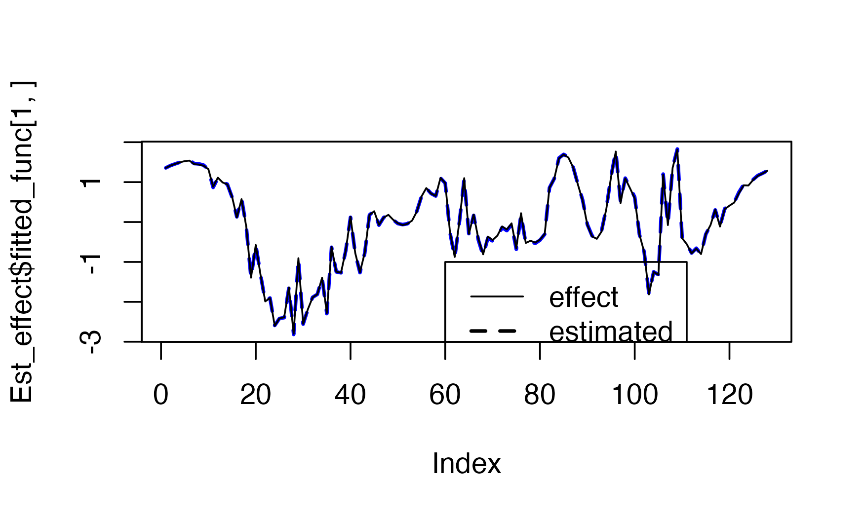
Y_corrected <-Est_effect$Y_adjustedYou can also perform the adjustment yourself by accessing the fitted curves directly (and potentially only removing the effect you are interested in)
  plot(  Y_corrected, Y-Cov %*%Est_effect$fitted_func,
         xlab = "output function",
         ylab="manual residualization")
Here, you can see that the corrected data closely matches the actual underlying signals.
par(mfrow=c(1,2))
plot( Y , target.data,pch=19,cex=.4,
      xlab="Observed data",
      ylab="Target data"
      )
plot( Y_corrected , target.data,pch=19,,cex=.4,
       xlab="Corrected data",
      ylab="Target data")
Fine-map
We can now fine-map our curves without to be worried of potential confounding due to population stratification or age
#> [1] "Scaling columns of X and Y to have unit variance"
#> [1] "Starting initialization"
#> [1] "Data transform"
#> [1] "Discarding  0 wavelet coefficients out of  128"
#> [1] "Data transform done"
#> [1] "Initializing prior"
#> [1] "Initialization done"
#> [1] "Fitting effect  1 , iter 1"
#> [1] "Fitting effect  2 , iter 1"
#> [1] "Fitting effect  3 , iter 1"
#> [1] "Adding  7  extra effects"
#> [1] "Fitting effect  1 , iter 2"
#> [1] "Fitting effect  2 , iter 2"
#> [1] "Fitting effect  3 , iter 2"
#> [1] "Fitting effect  4 , iter 2"
#> [1] "Fitting effect  5 , iter 2"
#> [1] "Fitting effect  6 , iter 2"
#> [1] "Fitting effect  7 , iter 2"
#> [1] "Fitting effect  8 , iter 2"
#> [1] "Fitting effect  9 , iter 2"
#> [1] "Fitting effect  10 , iter 2"
#> [1] "Discarding  0  effects"
#> [1] "Greedy search and backfitting done"
#> [1] "Fitting effect  1 , iter 3"
#> [1] "Fitting effect  2 , iter 3"
#> [1] "Fitting effect  3 , iter 3"
#> [1] "Fitting effect  4 , iter 3"
#> [1] "Fitting effect  5 , iter 3"
#> [1] "Fitting effect  6 , iter 3"
#> [1] "Fitting effect  7 , iter 3"
#> [1] "Fitting effect  8 , iter 3"
#> [1] "Fitting effect  9 , iter 3"
#> [1] "Fitting effect  10 , iter 3"
#> [1] "Fitting effect  1 , iter 4"
#> [1] "Fitting effect  2 , iter 4"
#> [1] "Fitting effect  3 , iter 4"
#> [1] "Fitting effect  4 , iter 4"
#> [1] "Fitting effect  5 , iter 4"
#> [1] "Fitting effect  6 , iter 4"
#> [1] "Fitting effect  7 , iter 4"
#> [1] "Fitting effect  8 , iter 4"
#> [1] "Fitting effect  9 , iter 4"
#> [1] "Fitting effect  10 , iter 4"
#> [1] "Fine mapping done, refining effect estimates using cylce spinning wavelet transform"
We can check the results
 plot_susiF(out)
#> $pip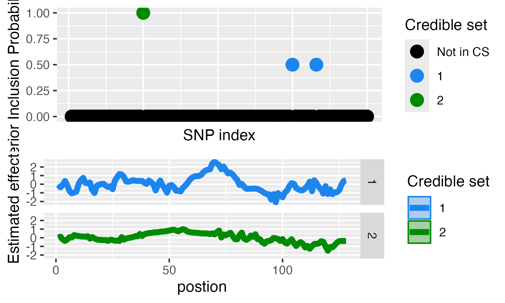
#>
#> $effect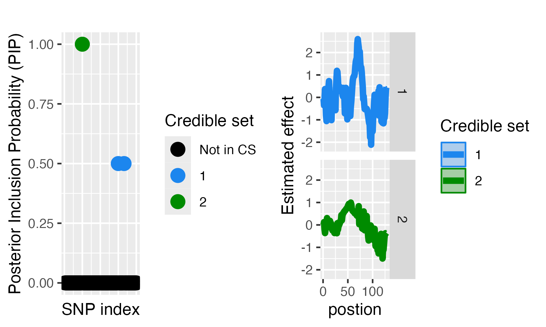
### Comparison with fine-mapping without adjustment
We can compare the performance when not adjusting.
#> [1] "Scaling columns of X and Y to have unit variance"
#> [1] "Starting initialization"
#> [1] "Data transform"
#> [1] "Discarding 0 wavelet coefficients out of 128"
#> [1] "Data transform done"
#> [1] "Initializing prior"
#> [1] "Initialization done"
#> [1] "Fitting effect 1 , iter 1"
#> [1] "Fitting effect 2 , iter 1"
#> [1] "Fitting effect 3 , iter 1"
#> [1] "Adding 7 extra effects"
#> [1] "Fitting effect 1 , iter 2"
#> [1] "Fitting effect 2 , iter 2"
#> [1] "Fitting effect 3 , iter 2"
#> [1] "Fitting effect 4 , iter 2"
#> [1] "Fitting effect 5 , iter 2"
#> [1] "Fitting effect 6 , iter 2"
#> [1] "Fitting effect 7 , iter 2"
#> [1] "Fitting effect 8 , iter 2"
#> [1] "Fitting effect 9 , iter 2"
#> [1] "Fitting effect 10 , iter 2"
#> [1] "Discarding 2 effects"
#> [1] "Fitting effect 1 , iter 3"
#> [1] "Fitting effect 2 , iter 3"
#> [1] "Fitting effect 3 , iter 3"
#> [1] "Fitting effect 4 , iter 3"
#> [1] "Fitting effect 5 , iter 3"
#> [1] "Fitting effect 6 , iter 3"
#> [1] "Fitting effect 7 , iter 3"
#> [1] "Fitting effect 8 , iter 3"
#> [1] "Discarding 2 effects"
#> [1] "Greedy search and backfitting done"
#> [1] "Fitting effect 1 , iter 4"
#> [1] "Fitting effect 2 , iter 4"
#> [1] "Fitting effect 3 , iter 4"
#> [1] "Fitting effect 4 , iter 4"
#> [1] "Fitting effect 5 , iter 4"
#> [1] "Fitting effect 6 , iter 4"
#> [1] "Fitting effect 7 , iter 4"
#> [1] "Fitting effect 8 , iter 4"
#> [1] "Fitting effect 1 , iter 5"
#> [1] "Fitting effect 2 , iter 5"
#> [1] "Fitting effect 3 , iter 5"
#> [1] "Fitting effect 4 , iter 5"
#> [1] "Fitting effect 5 , iter 5"
#> [1] "Fitting effect 6 , iter 5"
#> [1] "Fitting effect 7 , iter 5"
#> [1] "Fitting effect 8 , iter 5"
#> [1] "Fitting effect 1 , iter 6"
#> [1] "Fitting effect 2 , iter 6"
#> [1] "Fitting effect 3 , iter 6"
#> [1] "Fitting effect 4 , iter 6"
#> [1] "Fitting effect 5 , iter 6"
#> [1] "Fitting effect 6 , iter 6"
#> [1] "Fitting effect 7 , iter 6"
#> [1] "Fitting effect 8 , iter 6"
#> [1] "Fitting effect 1 , iter 7"
#> [1] "Fitting effect 2 , iter 7"
#> [1] "Fitting effect 3 , iter 7"
#> [1] "Fitting effect 4 , iter 7"
#> [1] "Fitting effect 5 , iter 7"
#> [1] "Fitting effect 6 , iter 7"
#> [1] "Fitting effect 7 , iter 7"
#> [1] "Fitting effect 8 , iter 7"
#> [1] "Fitting effect 1 , iter 8"
#> [1] "Fitting effect 2 , iter 8"
#> [1] "Fitting effect 3 , iter 8"
#> [1] "Fitting effect 4 , iter 8"
#> [1] "Fitting effect 5 , iter 8"
#> [1] "Fitting effect 6 , iter 8"
#> [1] "Fitting effect 7 , iter 8"
#> [1] "Fitting effect 8 , iter 8"
#> [1] "Fitting effect 1 , iter 9"
#> [1] "Fitting effect 2 , iter 9"
#> [1] "Fitting effect 3 , iter 9"
#> [1] "Fitting effect 4 , iter 9"
#> [1] "Fitting effect 5 , iter 9"
#> [1] "Fitting effect 6 , iter 9"
#> [1] "Fitting effect 7 , iter 9"
#> [1] "Fitting effect 8 , iter 9"
#> [1] "Fitting effect 1 , iter 10"
#> [1] "Fitting effect 2 , iter 10"
#> [1] "Fitting effect 3 , iter 10"
#> [1] "Fitting effect 4 , iter 10"
#> [1] "Fitting effect 5 , iter 10"
#> [1] "Fitting effect 6 , iter 10"
#> [1] "Fitting effect 7 , iter 10"
#> [1] "Fitting effect 8 , iter 10"
#> [1] "Fitting effect 1 , iter 11"
#> [1] "Fitting effect 2 , iter 11"
#> [1] "Fitting effect 3 , iter 11"
#> [1] "Fitting effect 4 , iter 11"
#> [1] "Fitting effect 5 , iter 11"
#> [1] "Fitting effect 6 , iter 11"
#> [1] "Fitting effect 7 , iter 11"
#> [1] "Fitting effect 8 , iter 11"
#> [1] "Fitting effect 1 , iter 12"
#> [1] "Fitting effect 2 , iter 12"
#> [1] "Fitting effect 3 , iter 12"
#> [1] "Fitting effect 4 , iter 12"
#> [1] "Fitting effect 5 , iter 12"
#> [1] "Fitting effect 6 , iter 12"
#> [1] "Fitting effect 7 , iter 12"
#> [1] "Fitting effect 8 , iter 12"
#> [1] "Fitting effect 1 , iter 13"
#> [1] "Fitting effect 2 , iter 13"
#> [1] "Fitting effect 3 , iter 13"
#> [1] "Fitting effect 4 , iter 13"
#> [1] "Fitting effect 5 , iter 13"
#> [1] "Fitting effect 6 , iter 13"
#> [1] "Fitting effect 7 , iter 13"
#> [1] "Fitting effect 8 , iter 13"
#> [1] "Fitting effect 1 , iter 14"
#> [1] "Fitting effect 2 , iter 14"
#> [1] "Fitting effect 3 , iter 14"
#> [1] "Fitting effect 4 , iter 14"
#> [1] "Fitting effect 5 , iter 14"
#> [1] "Fitting effect 6 , iter 14"
#> [1] "Fitting effect 7 , iter 14"
#> [1] "Fitting effect 8 , iter 14"
#> [1] "Fitting effect 1 , iter 15"
#> [1] "Fitting effect 2 , iter 15"
#> [1] "Fitting effect 3 , iter 15"
#> [1] "Fitting effect 4 , iter 15"
#> [1] "Fitting effect 5 , iter 15"
#> [1] "Fitting effect 6 , iter 15"
#> [1] "Fitting effect 7 , iter 15"
#> [1] "Fitting effect 8 , iter 15"
#> [1] "Fitting effect 1 , iter 16"
#> [1] "Fitting effect 2 , iter 16"
#> [1] "Fitting effect 3 , iter 16"
#> [1] "Fitting effect 4 , iter 16"
#> [1] "Fitting effect 5 , iter 16"
#> [1] "Fitting effect 6 , iter 16"
#> [1] "Fitting effect 7 , iter 16"
#> [1] "Fitting effect 8 , iter 16"
#> [1] "Fitting effect 1 , iter 17"
#> [1] "Fitting effect 2 , iter 17"
#> [1] "Fitting effect 3 , iter 17"
#> [1] "Fitting effect 4 , iter 17"
#> [1] "Fitting effect 5 , iter 17"
#> [1] "Fitting effect 6 , iter 17"
#> [1] "Fitting effect 7 , iter 17"
#> [1] "Fitting effect 8 , iter 17"
#> [1] "Fitting effect 1 , iter 18"
#> [1] "Fitting effect 2 , iter 18"
#> [1] "Fitting effect 3 , iter 18"
#> [1] "Fitting effect 4 , iter 18"
#> [1] "Fitting effect 5 , iter 18"
#> [1] "Fitting effect 6 , iter 18"
#> [1] "Fitting effect 7 , iter 18"
#> [1] "Fitting effect 8 , iter 18"
#> [1] "Fitting effect 1 , iter 19"
#> [1] "Fitting effect 2 , iter 19"
#> [1] "Fitting effect 3 , iter 19"
#> [1] "Fitting effect 4 , iter 19"
#> [1] "Fitting effect 5 , iter 19"
#> [1] "Fitting effect 6 , iter 19"
#> [1] "Fitting effect 7 , iter 19"
#> [1] "Fitting effect 8 , iter 19"
#> [1] "Fitting effect 1 , iter 20"
#> [1] "Fitting effect 2 , iter 20"
#> [1] "Fitting effect 3 , iter 20"
#> [1] "Fitting effect 4 , iter 20"
#> [1] "Fitting effect 5 , iter 20"
#> [1] "Fitting effect 6 , iter 20"
#> [1] "Fitting effect 7 , iter 20"
#> [1] "Fitting effect 8 , iter 20"
#> [1] "Fitting effect 1 , iter 21"
#> [1] "Fitting effect 2 , iter 21"
#> [1] "Fitting effect 3 , iter 21"
#> [1] "Fitting effect 4 , iter 21"
#> [1] "Fitting effect 5 , iter 21"
#> [1] "Fitting effect 6 , iter 21"
#> [1] "Fitting effect 7 , iter 21"
#> [1] "Fitting effect 8 , iter 21"
#> [1] "Fitting effect 1 , iter 22"
#> [1] "Fitting effect 2 , iter 22"
#> [1] "Fitting effect 3 , iter 22"
#> [1] "Fitting effect 4 , iter 22"
#> [1] "Fitting effect 5 , iter 22"
#> [1] "Fitting effect 6 , iter 22"
#> [1] "Fitting effect 7 , iter 22"
#> [1] "Fitting effect 8 , iter 22"
#> [1] "Fitting effect 1 , iter 23"
#> [1] "Fitting effect 2 , iter 23"
#> [1] "Fitting effect 3 , iter 23"
#> [1] "Fitting effect 4 , iter 23"
#> [1] "Fitting effect 5 , iter 23"
#> [1] "Fitting effect 6 , iter 23"
#> [1] "Fitting effect 7 , iter 23"
#> [1] "Fitting effect 8 , iter 23"
#> [1] "Fitting effect 1 , iter 24"
#> [1] "Fitting effect 2 , iter 24"
#> [1] "Fitting effect 3 , iter 24"
#> [1] "Fitting effect 4 , iter 24"
#> [1] "Fitting effect 5 , iter 24"
#> [1] "Fitting effect 6 , iter 24"
#> [1] "Fitting effect 7 , iter 24"
#> [1] "Fitting effect 8 , iter 24"
#> [1] "Fitting effect 1 , iter 25"
#> [1] "Fitting effect 2 , iter 25"
#> [1] "Fitting effect 3 , iter 25"
#> [1] "Fitting effect 4 , iter 25"
#> [1] "Fitting effect 5 , iter 25"
#> [1] "Fitting effect 6 , iter 25"
#> [1] "Fitting effect 7 , iter 25"
#> [1] "Fitting effect 8 , iter 25"
#> [1] "Fitting effect 1 , iter 26"
#> [1] "Fitting effect 2 , iter 26"
#> [1] "Fitting effect 3 , iter 26"
#> [1] "Fitting effect 4 , iter 26"
#> [1] "Fitting effect 5 , iter 26"
#> [1] "Fitting effect 6 , iter 26"
#> [1] "Fitting effect 7 , iter 26"
#> [1] "Fitting effect 8 , iter 26"
#> [1] "Fitting effect 1 , iter 27"
#> [1] "Fitting effect 2 , iter 27"
#> [1] "Fitting effect 3 , iter 27"
#> [1] "Fitting effect 4 , iter 27"
#> [1] "Fitting effect 5 , iter 27"
#> [1] "Fitting effect 6 , iter 27"
#> [1] "Fitting effect 7 , iter 27"
#> [1] "Fitting effect 8 , iter 27"
#> [1] "Fitting effect 1 , iter 28"
#> [1] "Fitting effect 2 , iter 28"
#> [1] "Fitting effect 3 , iter 28"
#> [1] "Fitting effect 4 , iter 28"
#> [1] "Fitting effect 5 , iter 28"
#> [1] "Fitting effect 6 , iter 28"
#> [1] "Fitting effect 7 , iter 28"
#> [1] "Fitting effect 8 , iter 28"
#> [1] "Fitting effect 1 , iter 29"
#> [1] "Fitting effect 2 , iter 29"
#> [1] "Fitting effect 3 , iter 29"
#> [1] "Fitting effect 4 , iter 29"
#> [1] "Fitting effect 5 , iter 29"
#> [1] "Fitting effect 6 , iter 29"
#> [1] "Fitting effect 7 , iter 29"
#> [1] "Fitting effect 8 , iter 29"
#> [1] "Fitting effect 1 , iter 30"
#> [1] "Fitting effect 2 , iter 30"
#> [1] "Fitting effect 3 , iter 30"
#> [1] "Fitting effect 4 , iter 30"
#> [1] "Fitting effect 5 , iter 30"
#> [1] "Fitting effect 6 , iter 30"
#> [1] "Fitting effect 7 , iter 30"
#> [1] "Fitting effect 8 , iter 30"
#> [1] "Fitting effect 1 , iter 31"
#> [1] "Fitting effect 2 , iter 31"
#> [1] "Fitting effect 3 , iter 31"
#> [1] "Fitting effect 4 , iter 31"
#> [1] "Fitting effect 5 , iter 31"
#> [1] "Fitting effect 6 , iter 31"
#> [1] "Fitting effect 7 , iter 31"
#> [1] "Fitting effect 8 , iter 31"
#> [1] "Fitting effect 1 , iter 32"
#> [1] "Fitting effect 2 , iter 32"
#> [1] "Fitting effect 3 , iter 32"
#> [1] "Fitting effect 4 , iter 32"
#> [1] "Fitting effect 5 , iter 32"
#> [1] "Fitting effect 6 , iter 32"
#> [1] "Fitting effect 7 , iter 32"
#> [1] "Fitting effect 8 , iter 32"
#> [1] "Fitting effect 1 , iter 33"
#> [1] "Fitting effect 2 , iter 33"
#> [1] "Fitting effect 3 , iter 33"
#> [1] "Fitting effect 4 , iter 33"
#> [1] "Fitting effect 5 , iter 33"
#> [1] "Fitting effect 6 , iter 33"
#> [1] "Fitting effect 7 , iter 33"
#> [1] "Fitting effect 8 , iter 33"
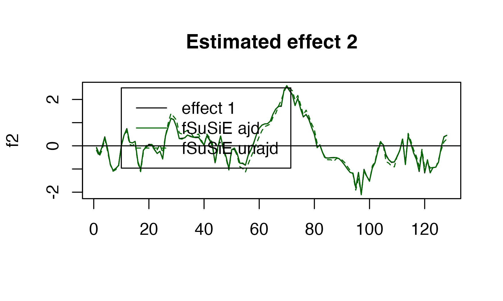
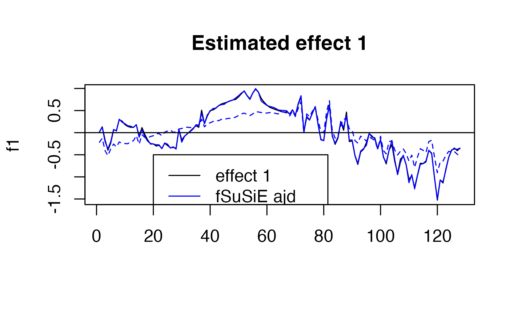
#> [1] "Fine mapping done, refining effect estimates using cylce spinning wavelet transform"Here we can see the performance.
 plot( f1,
       type="l",
       main="Estimated effect 1",
       xlab="")
 lines(get_fitted_effect(out,l=2),col='blue' )
 lines(get_fitted_effect(out_unadj,l=2),col='blue' , lty=2)

 abline(a=0,b=0)
 legend(x= 20,
        y=-0.5,
        lty= c(1,1,2),
        legend = c("effect 1","fSuSiE ajd", "fSuSiE unajd " ),
        col=c("black","blue","blue" )
 )
 plot( f2, type="l", main="Estimated effect 2", xlab="")
 lines(get_fitted_effect(out,l=1),col='darkgreen' )
 lines(get_fitted_effect(out_unadj,l=1),col='darkgreen' , lty=2)

 abline(a=0,b=0)
 legend(x= 10,
        y=2.5,
        lty= c(1,1,2),
        legend = c("effect 1","fSuSiE ajd", "fSuSiE unajd " ),
        col=c("black","darkgreen","darkgreen" )
 )