Low-dimensional Embeddings from Poisson NMF or Multinomial Topic Model

Lightweight interface for rapidly producing low-dimensional embeddings from matrix factorizations or multinomial topic models. The defaults used are more suitable for producing embeddings from matrix factorizations or topic models.

pca_from_topics(fit, dims = 2, center = TRUE, scale. = FALSE, ...)

tsne_from_topics(
  fit,
  dims = 2,
  pca = FALSE,
  normalize = FALSE,
  perplexity = 100,
  theta = 0.1,
  max_iter = 1000,
  eta = 200,
  check_duplicates = FALSE,
  verbose = TRUE,
  ...
)

umap_from_topics(
  fit,
  dims = 2,
  n_neighbors = 30,
  metric = "euclidean",
  scale = "none",
  pca = NULL,
  verbose = TRUE,
  ...
)

Arguments

fit

An object of class “poisson_nmf_fit” or “multinom_topic_model_fit”.

dims

The number of dimensions in the embedding. In tsne_from_topics, this is passed as argument “dims” to Rtsne. In umap_from_topics, this is passed as argument “n_components” to umap.

center

A logical value indicating whether columns of fit$L should be zero-centered before performing PCA; passed as argument “center” to prcomp.

scale.

A logical value indicating whether columns of fit$L should be scaled to have unit variance prior to performing PCA; passed as argument “scale.” to prcomp.

...

Additional arguments passed to prcomp, Rtsne or umap.

pca

Whether to perform a PCA processing step in t-SNE or UMAP; passed as argument “pca” to Rtsne or umap.

normalize

Whether to normalize the data prior to running t-SNE; passed as argument “normalize” to Rtsne.

perplexity

t-SNE perplexity parameter, passed as argument “perplexity” to Rtsne. The perplexity is automatically revised if it is too large; see Rtsne for more information.

theta

t-SNE speed/accuracy trade-off parameter; passed as argument “theta” to Rtsne.

max_iter

Maximum number of t-SNE iterations; passed as argument “max_iter” to Rtsne.

eta

t-SNE learning rate parameter; passed as argument “eta” to Rtsne.

check_duplicates

When check_duplicates = TRUE, checks whether there are duplicate rows in fit$L; passed as argument “check_duplicates” to Rtsne.

verbose

If verbose = TRUE, progress updates are printed; passed as argument “verbose” to Rtsne or umap.

n_neighbors

Number of nearest neighbours in manifold approximation; passed as argument “n_neighbors” to umap.

metric

Distance matrix used to find nearest neighbors; passed as argument “metric” to umap.

scale

Scaling to apply to fit$L; passed as argument “scale” to umap.

Value

An n x d matrix containing the embedding, where n is the number of rows of fit$L, and d = dims.

Details

Note that since tsne_from_topics and umap_from_topics use nonlinear transformations of the data, distances between points are generally less interpretable than a linear transformation obtained by, say, PCA.

References

Kobak, D. and Berens, P. (2019). The art of using t-SNE for single-cell transcriptomics. Nature Communications 10, 5416. doi:10.1038/s41467-019-13056-x

See also

pca_plot, tsne_plot, umap_plot, prcomp, Rtsne, umap

Examples

library(ggplot2)
library(cowplot)
set.seed(1)
data(pbmc_facs)

# Get the Poisson NMF and multinomial topic model fit to the PBMC data.
fit1 <- multinom2poisson(pbmc_facs$fit)
fit2 <- pbmc_facs$fit
fit2 <- poisson2multinom(fit1)

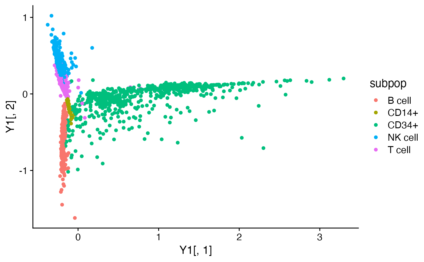
# Compute the first two PCs of the loadings matrix (for the topic
# model, fit2, the loadings are the topic proportions).
Y1 <- pca_from_topics(fit1)
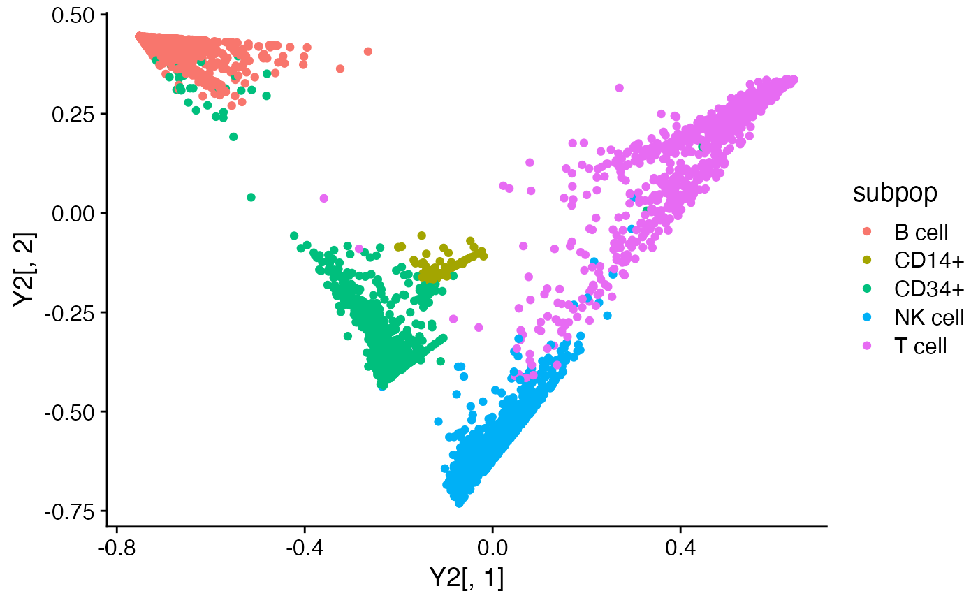
Y2 <- pca_from_topics(fit2)
subpop <- pbmc_facs$samples$subpop
quickplot(Y1[,1],Y1[,2],color = subpop) + theme_cowplot()
#> Warning: `qplot()` was deprecated in ggplot2 3.4.0.

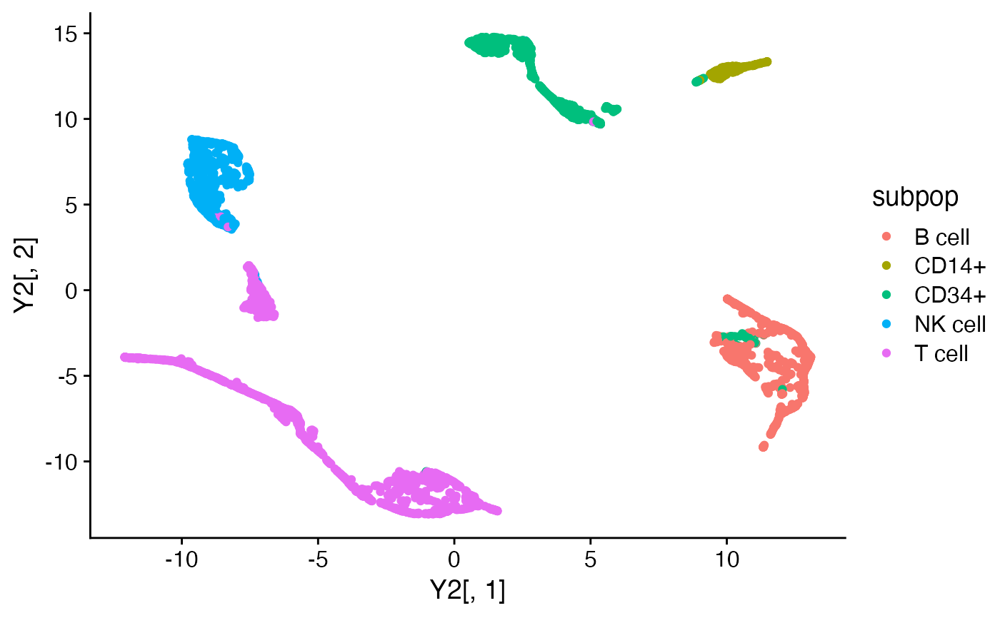
quickplot(Y2[,1],Y2[,2],color = subpop) + theme_cowplot()


# Compute a 2-d embedding of the loadings using t-SNE.
# \donttest{
Y1 <- tsne_from_topics(fit1)
#> Read the 3774 x 6 data matrix successfully!
#> Using no_dims = 2, perplexity = 100.000000, and theta = 0.100000
#> Computing input similarities...
#> Building tree...
#> Done in 0.97 seconds (sparsity = 0.103577)!
#> Learning embedding...
#> Iteration 50: error is 67.907680 (50 iterations in 2.31 seconds)
#> Iteration 100: error is 55.093036 (50 iterations in 1.63 seconds)
#> Iteration 150: error is 53.522705 (50 iterations in 1.56 seconds)
#> Iteration 200: error is 52.982723 (50 iterations in 1.54 seconds)
#> Iteration 250: error is 52.700813 (50 iterations in 1.54 seconds)
#> Iteration 300: error is 0.869868 (50 iterations in 1.89 seconds)
#> Iteration 350: error is 0.639018 (50 iterations in 2.04 seconds)
#> Iteration 400: error is 0.537143 (50 iterations in 2.01 seconds)
#> Iteration 450: error is 0.482721 (50 iterations in 2.01 seconds)
#> Iteration 500: error is 0.449646 (50 iterations in 1.98 seconds)
#> Iteration 550: error is 0.427580 (50 iterations in 1.97 seconds)
#> Iteration 600: error is 0.412004 (50 iterations in 1.95 seconds)
#> Iteration 650: error is 0.400458 (50 iterations in 1.93 seconds)
#> Iteration 700: error is 0.391642 (50 iterations in 1.95 seconds)
#> Iteration 750: error is 0.384759 (50 iterations in 1.96 seconds)
#> Iteration 800: error is 0.379201 (50 iterations in 1.97 seconds)
#> Iteration 850: error is 0.374679 (50 iterations in 1.97 seconds)
#> Iteration 900: error is 0.370959 (50 iterations in 1.98 seconds)
#> Iteration 950: error is 0.367860 (50 iterations in 2.10 seconds)
#> Iteration 1000: error is 0.365237 (50 iterations in 1.97 seconds)
#> Fitting performed in 38.27 seconds.
Y2 <- tsne_from_topics(fit2)
#> Read the 3774 x 6 data matrix successfully!
#> Using no_dims = 2, perplexity = 100.000000, and theta = 0.100000
#> Computing input similarities...
#> Building tree...
#> Done in 0.98 seconds (sparsity = 0.101133)!
#> Learning embedding...
#> Iteration 50: error is 65.682366 (50 iterations in 2.66 seconds)
#> Iteration 100: error is 53.576821 (50 iterations in 1.66 seconds)
#> Iteration 150: error is 51.735807 (50 iterations in 1.52 seconds)
#> Iteration 200: error is 51.078410 (50 iterations in 1.45 seconds)
#> Iteration 250: error is 50.736216 (50 iterations in 1.43 seconds)
#> Iteration 300: error is 0.804715 (50 iterations in 1.77 seconds)
#> Iteration 350: error is 0.580748 (50 iterations in 1.85 seconds)
#> Iteration 400: error is 0.481837 (50 iterations in 1.83 seconds)
#> Iteration 450: error is 0.429849 (50 iterations in 1.81 seconds)
#> Iteration 500: error is 0.398384 (50 iterations in 1.81 seconds)
#> Iteration 550: error is 0.377602 (50 iterations in 1.81 seconds)
#> Iteration 600: error is 0.362985 (50 iterations in 1.81 seconds)
#> Iteration 650: error is 0.352226 (50 iterations in 1.81 seconds)
#> Iteration 700: error is 0.344063 (50 iterations in 1.77 seconds)
#> Iteration 750: error is 0.337688 (50 iterations in 1.75 seconds)
#> Iteration 800: error is 0.332612 (50 iterations in 1.74 seconds)
#> Iteration 850: error is 0.328442 (50 iterations in 1.74 seconds)
#> Iteration 900: error is 0.325026 (50 iterations in 1.74 seconds)
#> Iteration 950: error is 0.322085 (50 iterations in 1.73 seconds)
#> Iteration 1000: error is 0.319664 (50 iterations in 1.72 seconds)
#> Fitting performed in 35.44 seconds.
quickplot(Y1[,1],Y1[,2],color = subpop) + theme_cowplot()

quickplot(Y2[,1],Y2[,2],color = subpop) + theme_cowplot()

# }

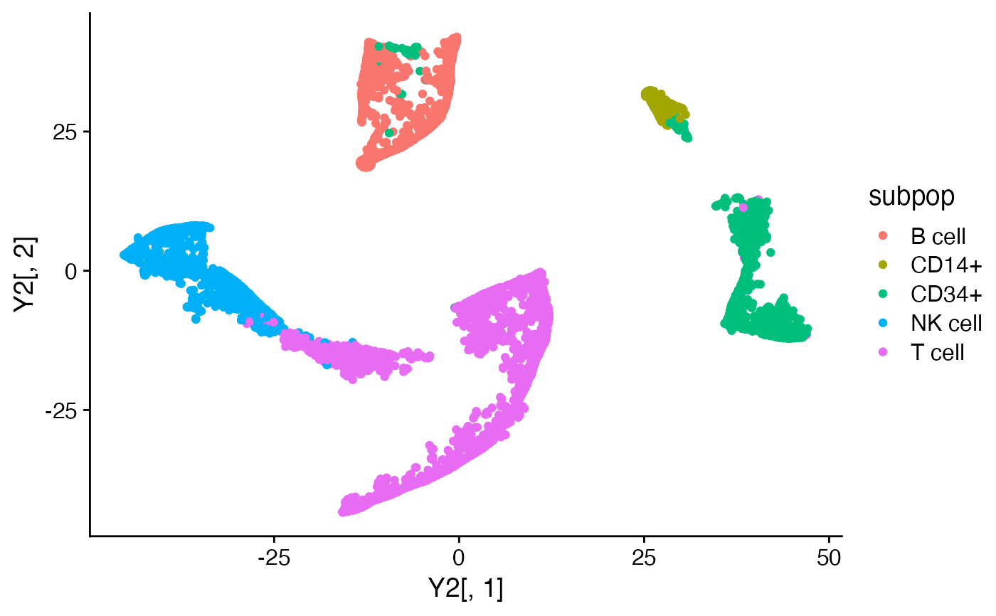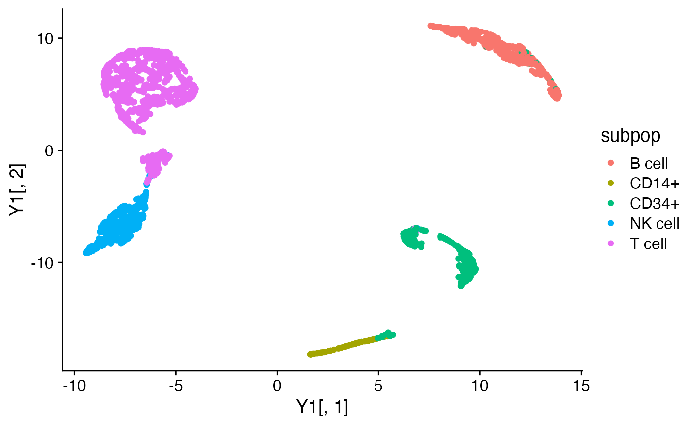
# Compute a 2-d embedding of the loadings using UMAP.
# \donttest{
Y1 <- umap_from_topics(fit1)
#> 09:22:32 UMAP embedding parameters a = 1.896 b = 0.8006
#> 09:22:32 Read 3774 rows and found 6 numeric columns
#> 09:22:32 Using FNN for neighbor search, n_neighbors = 30
#> 09:22:32 Commencing smooth kNN distance calibration using 4 threads
#>  with target n_neighbors = 30
#> 09:22:32 Initializing from normalized Laplacian + noise (using irlba)
#> 09:22:33 Commencing optimization for 500 epochs, with 139662 positive edges
#> 09:22:37 Optimization finished
Y2 <- umap_from_topics(fit2)
#> 09:22:37 UMAP embedding parameters a = 1.896 b = 0.8006
#> 09:22:37 Read 3774 rows and found 6 numeric columns
#> 09:22:37 Using FNN for neighbor search, n_neighbors = 30
#> 09:22:38 Commencing smooth kNN distance calibration using 4 threads
#>  with target n_neighbors = 30
#> 09:22:38 110 smooth knn distance failures
#> 09:22:38 Initializing from normalized Laplacian + noise (using irlba)
#> 09:22:38 Commencing optimization for 500 epochs, with 137990 positive edges
#> 09:22:43 Optimization finished
quickplot(Y1[,1],Y1[,2],color = subpop) + theme_cowplot()

quickplot(Y2[,1],Y2[,2],color = subpop) + theme_cowplot()

# }