This function implements empirical Bayes methods for fitting a multivariate version of the normal means model with flexible prior. These methods are closely related to approaches for multivariate density deconvolution (Sarkar et al, 2018), so it can also be viewed as a method for multivariate density deconvolution.
ud_fit(fit, X, control = list(), verbose = TRUE)

ud_fit_control_default()
Arguments
- fit
A previous Ultimate Deconvolution model fit. Typically, this will be an output of
ud_initor an output from a previous call toud_fit.- X
Optional n x m data matrix, in which each row of the matrix is an m-dimensional data point. The number of rows and columns should be 2 or more. When not provided,
fit$Xis used.- control
A list of parameters controlling the behaviour of the model fitting and initialization. See ‘Details’.
- verbose
When
verbose = TRUE, information about the algorithm's progress is printed to the console at each iteration. For interpretation of the columns, see the description of theprogressreturn value.
Value
An Ultimate Deconvolution model fit. It is a list object with the following elements:
- X
The data matrix used to fix the model.
- w
A vector containing the estimated mixture weights \(w\)
- U
A list containing the estimated prior covariance matrices \(U\)
- V
The residual covariance matrix \(V\), or a list of \(V_j\) used in the model fit.
- P
The responsibilities matrix in which
P[i,j]is the posterior mixture probability for data point i and mixture component j.- loglik
The log-likelihood at the current settings of the model parameters.
- progress
A data frame containing detailed information about the algorithm's progress. The columns of the data frame are: "iter", the iteration number; "loglik", the log-likelihood at the current estimates of the model parameters; "loglik.pen", the penalized log-likelihood at the current estimates of the model parameters. It is equal to "loglik" when no covariance regularization is used. "delta.w", the largest change in the mixture weights; "delta.u", the largest change in the prior covariance matrices; "delta.v", the largest change in the residual covariance matrix; and "timing", the elapsed time in seconds (recorded using
proc.time).
Details
The udr package fits the following Empirical Bayes version of the multivariate normal means model:
Independently for \(j=1,\dots,n\),
\(x_j | \theta_j, V_j ~ N_m(\theta_j, V_j)\);
\(\theta_j | V_j ~ w_1 N_m(0, U_1) + \dots + w_K N_m(0,U_K)\).
Here the variances \(V_j\) are usually considered known, and may be equal (\(V_j=V\)) which can greatly simplify computation. The prior on \(theta_j\) is a mixture of \(K \ge 2\) multivariate normals, with unknown mixture proportions \(w=(w_1,...,w_K)\) and covariance matrices \(U=(U_1,...,U_K)\). We call this the ``Ultimate Deconvolution" (UD) model.
Fitting the UD model involves i) obtaining maximum likelihood estimates \(\hat{w}\) and \(\hat{U}\) for the prior parameters \(w\) and \(U\); ii) computing the posterior distributions \(p(\theta_j | x_j, \hat{w}, \hat{U})\).
The UD model is fit by an iterative expectation-maximization (EM)-based algorithm. Various algorithms are implemented to deal with different constraints on each \(U_k\). Specifically, each \(U_k\) can be i) constrained to be a scalar multiple of a pre-specified matrix; or ii) constrained to be a rank-1 matrix; or iii) unconstrained. How many mixture components to use and which constraints to apply to each \(U_k\) are specified using ud_init.
In addition, we introduced two covariance regularization approaches to handle the high dimensional challenges, where sample size is relatively small compared with data dimension. One is called nucler norm regularization, short for "nu". The other is called inverse-Wishart regularization, short for "iw".
The control argument can be used to adjust the algorithm
settings, although the default settings should suffice for most users.
It is a list in which any of the following named components
will override the default algorithm settings (as they are defined
by ud_fit_control_default):
weights.updateWhen
weights.update = "em", the mixture weights are updated via EM; whenweights.update = "none", the mixture weights are not updated.resid.updateWhen
resid.update = "em", the residual covariance matrix \(V\) is updated via an EM step; this option is experimental, not tested and not recommended. Whenresid.update = "none", the residual covariance matrices \(V\) is not updated.scaled.updateThis setting specifies the updates for the scaled prior covariance matrices. Possible settings are
"fa","none"orNA.rank1.updateThis setting specifies the updates for the rank-1 prior covariance matrices. Possible settings are
"ed","ted","none"orNA.unconstrained.updateThis setting determines the updates used to estimate the unconstrained prior covariance matrices. Two variants of EM are implemented:
update.U =
"ed"
, the EM updates described by Bovy et al (2011); andupdate.U = "ted", "truncated eigenvalue decomposition", in which the M-step update for each covariance matrixU[[j]]is solved by truncating the eigenvalues in a spectral decomposition of the unconstrained maximimum likelihood estimate (MLE) ofU[[j]]. Other possible settings include"none"or codeNA.versionR and C++ implementations of the model fitting algorithm are provided; these are selected with
version = "R"andversion = "Rcpp".maxiterThe upper limit on the number of updates to perform.
tolThe updates are halted when the largest change in the model parameters between two successive updates is less than
tol.tol.likThe updates are halted when the change in increase in the likelihood between two successive iterations is less than
tol.lik.minvalMinimum eigenvalue allowed in the residual covariance(s)
Vand the prior covariance matricesU. Should be a small, positive number.update.thresholdA prior covariance matrix
U[[i]]is only updated if the total “responsibility” for componentiexceedsupdate.threshold; that is, only ifsum(P[,i]) > update.threshold.lambdaParameter to control the strength of covariance regularization.
lambda = 0indicates no covariance regularization.penalty.typeSpecifies the type of covariance regularization to use. "iw": inverse Wishart regularization, "nu": nuclear norm regularization.
Using this function requires some care; currently only minimal argument checking is performed. See the documentation and examples for guidance.
References
J. Bovy, D. W. Hogg and S. T. Roweis (2011). Extreme Deconvolution: inferring complete distribution functions from noisy, heterogeneous and incomplete observations. Annals of Applied Statistics, 5, 1657???1677. doi:10.1214/10-AOAS439
D. B. Rubin and D. T. Thayer (1982). EM algorithms for ML factor analysis. Psychometrika 47, 69-76. doi:10.1007/BF02293851
A. Sarkar, D. Pati, A. Chakraborty, B. K. Mallick and R. J. Carroll (2018). Bayesian semiparametric multivariate density deconvolution. Journal of the American Statistical Association 113, 401???416. doi:10.1080/01621459.2016.1260467
J. Won, J. Lim, S. Kim and B. Rajaratnam (2013). Condition-number-regularized covariance estimation. Journal of the Royal Statistical Society, Series B 75, 427???450. doi:10.1111/j.1467-9868.2012.01049.x
Examples
# Simulate data from a UD model.
set.seed(1)
n <- 4000
V <- rbind(c(0.8,0.2),
c(0.2,1.5))
U <- list(none = rbind(c(0,0),
c(0,0)),
shared = rbind(c(1.0,0.9),
c(0.9,1.0)),
only1 = rbind(c(1,0),
c(0,0)),
only2 = rbind(c(0,0),
c(0,1)))
w <- c(0.8,0.1,0.075,0.025)
rownames(V) <- c("d1","d2")
colnames(V) <- c("d1","d2")
X <- simulate_ud_data(n,w,U,V)
# This is the simplest invocation of ud_init and ud_fit.
# It uses the default settings for the prior
# (which are 2 scaled components, 4 rank-1 components, and 4 unconstrained components)
fit1 <- ud_init(X,V = V)
fit1 <- ud_fit(fit1)
#> Performing Ultimate Deconvolution on 4000 x 2 matrix (udr 0.3-152, "R"):
#> data points are i.i.d. (same V)
#> prior covariances: 2 scaled, 0 rank-1, 8 unconstrained
#> prior covariance updates: scaled (fa), rank-1 (none), unconstrained (ted)
#> covariance regularization: penalty strength = 0.00e+00, method = iw
#> mixture weights update: em
#> residual covariance update: none
#> max 20 updates, tol=1.0e-06, tol.lik=1.0e-03
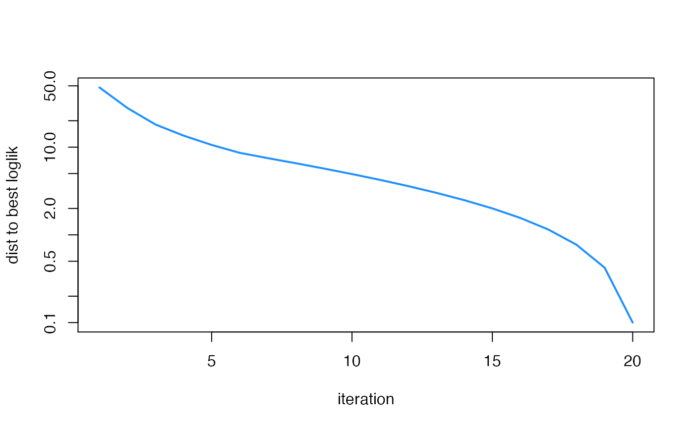
#> iter log-likelihood log-likelihood.pen |w - w'| |U - U'| |V - V'|
#> 1 -1.2279804719045842e+04 -1.2279804719045842e+04 4.68e-02 1.28e+01 0.00e+00
#> 2 -1.2223122563101466e+04 -1.2223122563101466e+04 8.81e-03 5.10e-01 0.00e+00
#> 3 -1.2212191560680643e+04 -1.2212191560680643e+04 6.38e-03 1.89e-01 0.00e+00
#> 4 -1.2208916818919344e+04 -1.2208916818919344e+04 4.86e-03 8.34e-02 0.00e+00
#> 5 -1.2207216863575988e+04 -1.2207216863575988e+04 4.05e-03 4.79e-02 0.00e+00
#> 6 -1.2206156766378293e+04 -1.2206156766378293e+04 3.50e-03 3.68e-02 0.00e+00
#> 7 -1.2205421131712248e+04 -1.2205421131712248e+04 3.08e-03 3.03e-02 0.00e+00
#> 8 -1.2204896399982579e+04 -1.2204896399982579e+04 2.74e-03 2.46e-02 0.00e+00
#> 9 -1.2204481866400763e+04 -1.2204481866400763e+04 2.48e-03 1.95e-02 0.00e+00
#> 10 -1.2204146935386652e+04 -1.2204146935386652e+04 2.26e-03 1.51e-02 0.00e+00
#> 11 -1.2203870133940494e+04 -1.2203870133940494e+04 2.07e-03 1.14e-02 0.00e+00
#> 12 -1.2203634530812882e+04 -1.2203634530812882e+04 1.91e-03 8.30e-03 0.00e+00
#> 13 -1.2203423288928794e+04 -1.2203423288928794e+04 1.78e-03 5.97e-03 0.00e+00
#> 14 -1.2203229520596969e+04 -1.2203229520596969e+04 1.67e-03 4.45e-03 0.00e+00
#> 15 -1.2203050854108164e+04 -1.2203050854108164e+04 1.59e-03 3.40e-03 0.00e+00
#> 16 -1.2202885740594420e+04 -1.2202885740594420e+04 1.51e-03 2.64e-03 0.00e+00
#> 17 -1.2202732915230425e+04 -1.2202732915230425e+04 1.43e-03 2.23e-03 0.00e+00
#> 18 -1.2202591285909395e+04 -1.2202591285909395e+04 1.37e-03 2.09e-03 0.00e+00
#> 19 -1.2202459890830853e+04 -1.2202459890830853e+04 1.30e-03 1.98e-03 0.00e+00
#> 20 -1.2202337873657989e+04 -1.2202337873657989e+04 1.24e-03 1.89e-03 0.00e+00
logLik(fit1)
#> 'log Lik.' -12202 (df=NA)
summary(fit1)
#> Model overview:
#> Number of data points: 4000
#> Dimension of data points: 2
#> Data points are i.i.d. (same V)
#> Number of scaled prior covariances: 2
#> Number of rank-1 prior covariances: 0
#> Number of unconstrained prior covariances: 8
#> Evaluation of fit (20 updates performed):
#> Log-likelihood: -1.220233787366e+04
plot(fit1$progress$iter,
max(fit1$progress$loglik) - fit1$progress$loglik + 0.1,
type = "l",col = "dodgerblue",lwd = 2,log = "y",xlab = "iteration",
ylab = "dist to best loglik")
 # This is a more complex invocation of ud_init that overrides some
# of the defaults.
fit2 <- ud_init(X,U_scaled = U,n_rank1 = 1,n_unconstrained = 1,V = V)
fit2 <- ud_fit(fit2)
#> Performing Ultimate Deconvolution on 4000 x 2 matrix (udr 0.3-152, "R"):
#> data points are i.i.d. (same V)
#> prior covariances: 4 scaled, 1 rank-1, 1 unconstrained
#> prior covariance updates: scaled (fa), rank-1 (ted), unconstrained (ted)
#> covariance regularization: penalty strength = 0.00e+00, method = iw
#> mixture weights update: em
#> residual covariance update: none
#> max 20 updates, tol=1.0e-06, tol.lik=1.0e-03
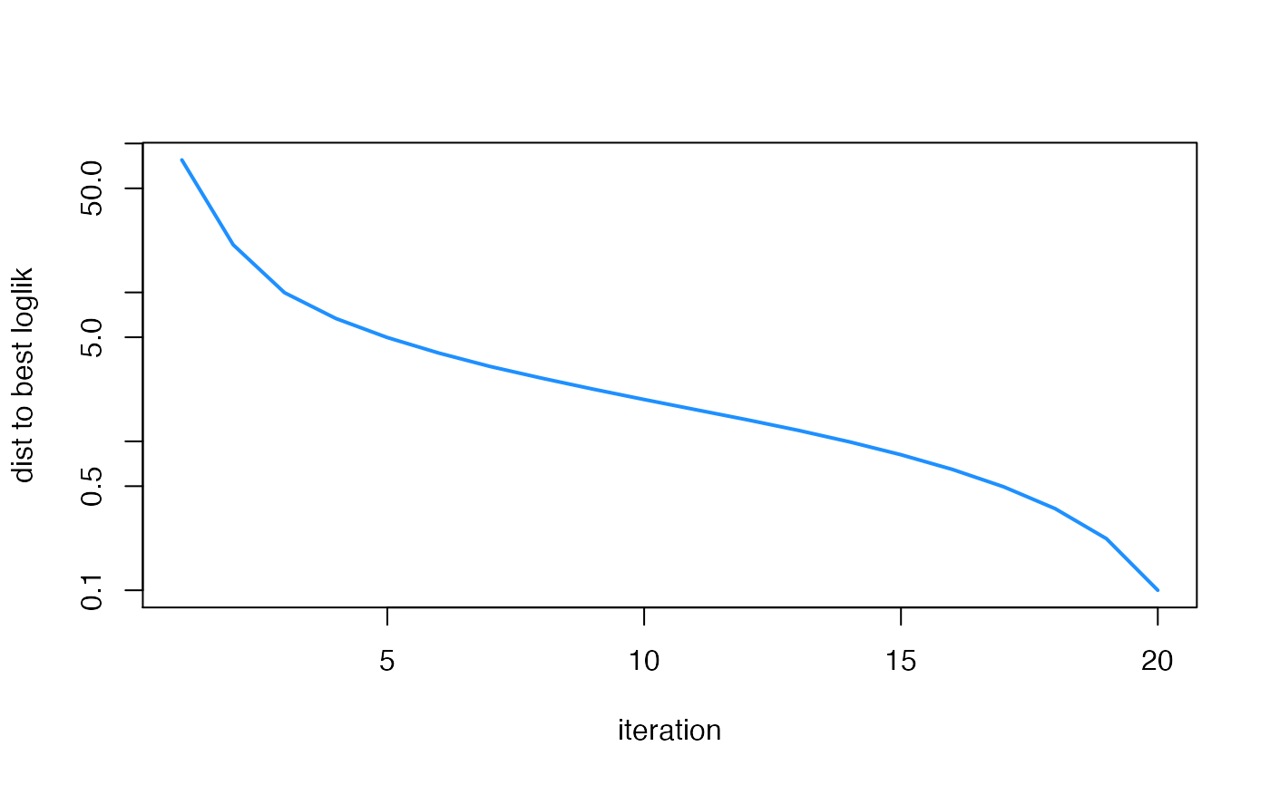
#> iter log-likelihood log-likelihood.pen |w - w'| |U - U'| |V - V'|
#> 1 -1.2254274362886588e+04 -1.2254274362886588e+04 2.15e-02 1.01e+00 0.00e+00
#> 2 -1.2234214947140643e+04 -1.2234214947140643e+04 7.12e-03 2.99e-01 0.00e+00
#> 3 -1.2224394571154378e+04 -1.2224394571154378e+04 5.32e-03 1.62e-01 0.00e+00
#> 4 -1.2219820969163555e+04 -1.2219820969163555e+04 4.73e-03 1.00e-01 0.00e+00
#> 5 -1.2216889114009215e+04 -1.2216889114009215e+04 4.15e-03 6.61e-02 0.00e+00
#> 6 -1.2214904923248048e+04 -1.2214904923248048e+04 3.61e-03 4.32e-02 0.00e+00
#> 7 -1.2213781656525432e+04 -1.2213781656525432e+04 3.12e-03 4.90e-03 0.00e+00
#> 8 -1.2212842079106016e+04 -1.2212842079106016e+04 2.83e-03 6.62e-24 0.00e+00
#> 9 -1.2211992244201772e+04 -1.2211992244201772e+04 2.66e-03 3.31e-24 0.00e+00
#> 10 -1.2211222160441317e+04 -1.2211222160441317e+04 2.53e-03 6.62e-24 0.00e+00
#> 11 -1.2210522990596364e+04 -1.2210522990596364e+04 2.41e-03 6.62e-24 0.00e+00
#> 12 -1.2209886923773960e+04 -1.2209886923773960e+04 2.30e-03 9.93e-24 0.00e+00
#> 13 -1.2209307059316559e+04 -1.2209307059316559e+04 2.19e-03 6.62e-24 0.00e+00
#> 14 -1.2208777302107714e+04 -1.2208777302107714e+04 2.09e-03 3.31e-24 0.00e+00
#> 15 -1.2208292268716075e+04 -1.2208292268716075e+04 2.07e-03 3.31e-24 0.00e+00
#> 16 -1.2207847203652633e+04 -1.2207847203652633e+04 2.06e-03 9.93e-24 0.00e+00
#> 17 -1.2207437904935397e+04 -1.2207437904935397e+04 2.04e-03 9.93e-24 0.00e+00
#> 18 -1.2207060658129330e+04 -1.2207060658129330e+04 2.02e-03 6.62e-24 0.00e+00
#> 19 -1.2206712178039492e+04 -1.2206712178039492e+04 2.00e-03 6.62e-24 0.00e+00
#> 20 -1.2206389557269531e+04 -1.2206389557269531e+04 1.97e-03 6.62e-24 0.00e+00
logLik(fit2)
#> 'log Lik.' -12206 (df=NA)
summary(fit2)
#> Model overview:
#> Number of data points: 4000
#> Dimension of data points: 2
#> Data points are i.i.d. (same V)
#> Number of scaled prior covariances: 4
#> Number of rank-1 prior covariances: 1
#> Number of unconstrained prior covariances: 1
#> Evaluation of fit (20 updates performed):
#> Log-likelihood: -1.220638955727e+04
plot(fit2$progress$iter,
max(fit2$progress$loglik) - fit2$progress$loglik + 0.1,
type = "l",col = "dodgerblue",lwd = 2,log = "y",xlab = "iteration",
ylab = "dist to best loglik")
# This is a more complex invocation of ud_init that overrides some
# of the defaults.
fit2 <- ud_init(X,U_scaled = U,n_rank1 = 1,n_unconstrained = 1,V = V)
fit2 <- ud_fit(fit2)
#> Performing Ultimate Deconvolution on 4000 x 2 matrix (udr 0.3-152, "R"):
#> data points are i.i.d. (same V)
#> prior covariances: 4 scaled, 1 rank-1, 1 unconstrained
#> prior covariance updates: scaled (fa), rank-1 (ted), unconstrained (ted)
#> covariance regularization: penalty strength = 0.00e+00, method = iw
#> mixture weights update: em
#> residual covariance update: none
#> max 20 updates, tol=1.0e-06, tol.lik=1.0e-03
#> iter log-likelihood log-likelihood.pen |w - w'| |U - U'| |V - V'|
#> 1 -1.2254274362886588e+04 -1.2254274362886588e+04 2.15e-02 1.01e+00 0.00e+00
#> 2 -1.2234214947140643e+04 -1.2234214947140643e+04 7.12e-03 2.99e-01 0.00e+00
#> 3 -1.2224394571154378e+04 -1.2224394571154378e+04 5.32e-03 1.62e-01 0.00e+00
#> 4 -1.2219820969163555e+04 -1.2219820969163555e+04 4.73e-03 1.00e-01 0.00e+00
#> 5 -1.2216889114009215e+04 -1.2216889114009215e+04 4.15e-03 6.61e-02 0.00e+00
#> 6 -1.2214904923248048e+04 -1.2214904923248048e+04 3.61e-03 4.32e-02 0.00e+00
#> 7 -1.2213781656525432e+04 -1.2213781656525432e+04 3.12e-03 4.90e-03 0.00e+00
#> 8 -1.2212842079106016e+04 -1.2212842079106016e+04 2.83e-03 6.62e-24 0.00e+00
#> 9 -1.2211992244201772e+04 -1.2211992244201772e+04 2.66e-03 3.31e-24 0.00e+00
#> 10 -1.2211222160441317e+04 -1.2211222160441317e+04 2.53e-03 6.62e-24 0.00e+00
#> 11 -1.2210522990596364e+04 -1.2210522990596364e+04 2.41e-03 6.62e-24 0.00e+00
#> 12 -1.2209886923773960e+04 -1.2209886923773960e+04 2.30e-03 9.93e-24 0.00e+00
#> 13 -1.2209307059316559e+04 -1.2209307059316559e+04 2.19e-03 6.62e-24 0.00e+00
#> 14 -1.2208777302107714e+04 -1.2208777302107714e+04 2.09e-03 3.31e-24 0.00e+00
#> 15 -1.2208292268716075e+04 -1.2208292268716075e+04 2.07e-03 3.31e-24 0.00e+00
#> 16 -1.2207847203652633e+04 -1.2207847203652633e+04 2.06e-03 9.93e-24 0.00e+00
#> 17 -1.2207437904935397e+04 -1.2207437904935397e+04 2.04e-03 9.93e-24 0.00e+00
#> 18 -1.2207060658129330e+04 -1.2207060658129330e+04 2.02e-03 6.62e-24 0.00e+00
#> 19 -1.2206712178039492e+04 -1.2206712178039492e+04 2.00e-03 6.62e-24 0.00e+00
#> 20 -1.2206389557269531e+04 -1.2206389557269531e+04 1.97e-03 6.62e-24 0.00e+00
logLik(fit2)
#> 'log Lik.' -12206 (df=NA)
summary(fit2)
#> Model overview:
#> Number of data points: 4000
#> Dimension of data points: 2
#> Data points are i.i.d. (same V)
#> Number of scaled prior covariances: 4
#> Number of rank-1 prior covariances: 1
#> Number of unconstrained prior covariances: 1
#> Evaluation of fit (20 updates performed):
#> Log-likelihood: -1.220638955727e+04
plot(fit2$progress$iter,
max(fit2$progress$loglik) - fit2$progress$loglik + 0.1,
type = "l",col = "dodgerblue",lwd = 2,log = "y",xlab = "iteration",
ylab = "dist to best loglik")