Simulate ridge regression using mean field method
Zhengyang Fang
June 27, 2019
Last updated: 2019-08-01
Checks: 7 0
Knit directory: susie-mixture/analysis/
This reproducible R Markdown analysis was created with workflowr (version 1.4.0). The Checks tab describes the reproducibility checks that were applied when the results were created. The Past versions tab lists the development history.
Great! Since the R Markdown file has been committed to the Git repository, you know the exact version of the code that produced these results.
Great job! The global environment was empty. Objects defined in the global environment can affect the analysis in your R Markdown file in unknown ways. For reproduciblity it’s best to always run the code in an empty environment.
The command set.seed(1) was run prior to running the code in the R Markdown file. Setting a seed ensures that any results that rely on randomness, e.g. subsampling or permutations, are reproducible.
Great job! Recording the operating system, R version, and package versions is critical for reproducibility.
Nice! There were no cached chunks for this analysis, so you can be confident that you successfully produced the results during this run.
Great job! Using relative paths to the files within your workflowr project makes it easier to run your code on other machines.
Great! You are using Git for version control. Tracking code development and connecting the code version to the results is critical for reproducibility. The version displayed above was the version of the Git repository at the time these results were generated.
Note that you need to be careful to ensure that all relevant files for the analysis have been committed to Git prior to generating the results (you can use wflow_publish or wflow_git_commit). workflowr only checks the R Markdown file, but you know if there are other scripts or data files that it depends on. Below is the status of the Git repository when the results were generated:
Ignored files:
    Ignored:    .RData
    Ignored:    .Rhistory
    Ignored:    .Rproj.user/
    Ignored:    analysis/.RData
    Ignored:    analysis/.Rhistory
Note that any generated files, e.g. HTML, png, CSS, etc., are not included in this status report because it is ok for generated content to have uncommitted changes.
These are the previous versions of the R Markdown and HTML files. If you’ve configured a remote Git repository (see ?wflow_git_remote), click on the hyperlinks in the table below to view them.
| File | Version | Author | Date | Message |
|---|---|---|---|---|
| html | 034283b | Zhengyang Fang | 2019-07-22 | Build site. |
| html | 6d9cbaa | Zhengyang Fang | 2019-07-22 | Build site. |
| html | 2a474f9 | Zhengyang Fang | 2019-07-22 | Build site. |
| html | c72a707 | Zhengyang Fang | 2019-07-22 | Build site. |
| html | 8092e5a | Zhengyang Fang | 2019-07-19 | Build site. |
| html | 5d3e3ef | Zhengyang Fang | 2019-07-11 | Build site. |
| html | 3eee187 | Zhengyang Fang | 2019-07-03 | Build site. |
| html | f303e14 | Zhengyang Fang | 2019-07-01 | Build site. |
| html | def2b27 | Zhengyang Fang | 2019-06-28 | Build site. |
| html | 05f778b | Zhengyang Fang | 2019-06-28 | Build site. |
| html | 38b5b82 | Zhengyang Fang | 2019-06-27 | Build site. |
| Rmd | 200b9d7 | Zhengyang Fang | 2019-06-27 | wflow_publish(“ridge_VI_vanilla.Rmd”) |
| html | 0d93bf5 | Zhengyang Fang | 2019-06-27 | Build site. |
| Rmd | 4bda68d | Zhengyang Fang | 2019-06-27 | wflow_publish(“ridge_VI_vanilla.Rmd”) |
I. Algorithm code
#' VI.ELBO: use VI to solve ridge regression, updating by directly maximizing ELBO
#' @param X: variables in linear model
#' @param Y: response in linear model
#' @param sigma.b: the variance of prior of coefficients
#' @return the posterior mean, result of ridge regression

VI.ELBO <- function (X, Y, sigma.b, max.iter = 300) {
    p <- ncol(X)
    n <- nrow(X)

    # intercept
    beta.hat <- numeric(p + 1)
    beta.hat[1] <- mean(Y)

    # center the columns of X and Y
    Y <- Y - mean(Y)
    X <- t(t(X) - colMeans(X))

    # preprocess to make it faster
    col.norm.sq <- colSums(X ^ 2)

    mu <- rep(0, p)

    converge <- FALSE
    iter <- 0
    while (!converge && iter < max.iter) {
        converge = TRUE
        iter <- iter + 1

        record.mu <- mu

        for (k in 1: p) {
            r <- Y - X[, -k] %*% mu[-k]
            mu[k] <- (t(r) %*% X[, k]) / (col.norm.sq[k] + 1 / (sigma.b ^ 2))
        }
        if (sum(abs(mu - record.mu)) > 1e-4)
            converge <- FALSE
    }

    beta.hat[2: (p + 1)] <- mu

    result <- list()
    result$coef <- beta.hat
    result$converge <- converge

    return (result)
}
II. A simple simulation
Generate data where elements in \(\textbf X\) are i.i.d Gaussian.
set.seed(1)

sigma   <- 3
sigma.b <- 0.5
p       <- 200
n       <- 300

true.beta <- rnorm (p, 0, sd = sigma.b * sigma)
X <- matrix (rnorm (n * p), nrow = n, ncol = p)
Y <- rnorm (n, X %*% true.beta + 1, sigma)
we compare VI with ridge regression, where the tuning parameter in ridge regression is chosen by cross-validation.
Ridge regression finds the exact posterior estimate, while VI only returns an approximation. We compare their result to see how this approximation works.
library(lasso2)
library(MASS)
library(glmnet)

#' compare: compare the result of ridge regression and VI, plot their estimate coefs
#' @param X: variables in linear model
#' @param Y: response in linear model
#' @return whether VI method converges

compare <- function (X, Y, p = 200, n = 300,
                     plot.title = 'VI (mean field) v.s. ridge regression') {
    cvfit <- cv.glmnet(X, Y, alpha = 0)
    lambda <- cvfit$lambda.1se

    # remove the intercept
    ridge.coef <- coef(cvfit, s = "lambda.1se")[2: (p + 1)]

    # choose sigma.b^2 = 1 / lambda, so that VI solves the same problem
    # as ridge regression
    VI.ELBO.result <- VI.ELBO(X, Y, sqrt(1 / lambda))

    # remove the intercept
    VI.ELBO.coef   <- VI.ELBO.result$coef[2: (p + 1)]

    plot (VI.ELBO.coef, ridge.coef,
          main = plot.title,
          xlab = 'VI coefficient', ylab = 'ridge coefficient')
    abline(a = 0, b = 1)

    return (VI.ELBO.result$converge)
}

compare(X, Y)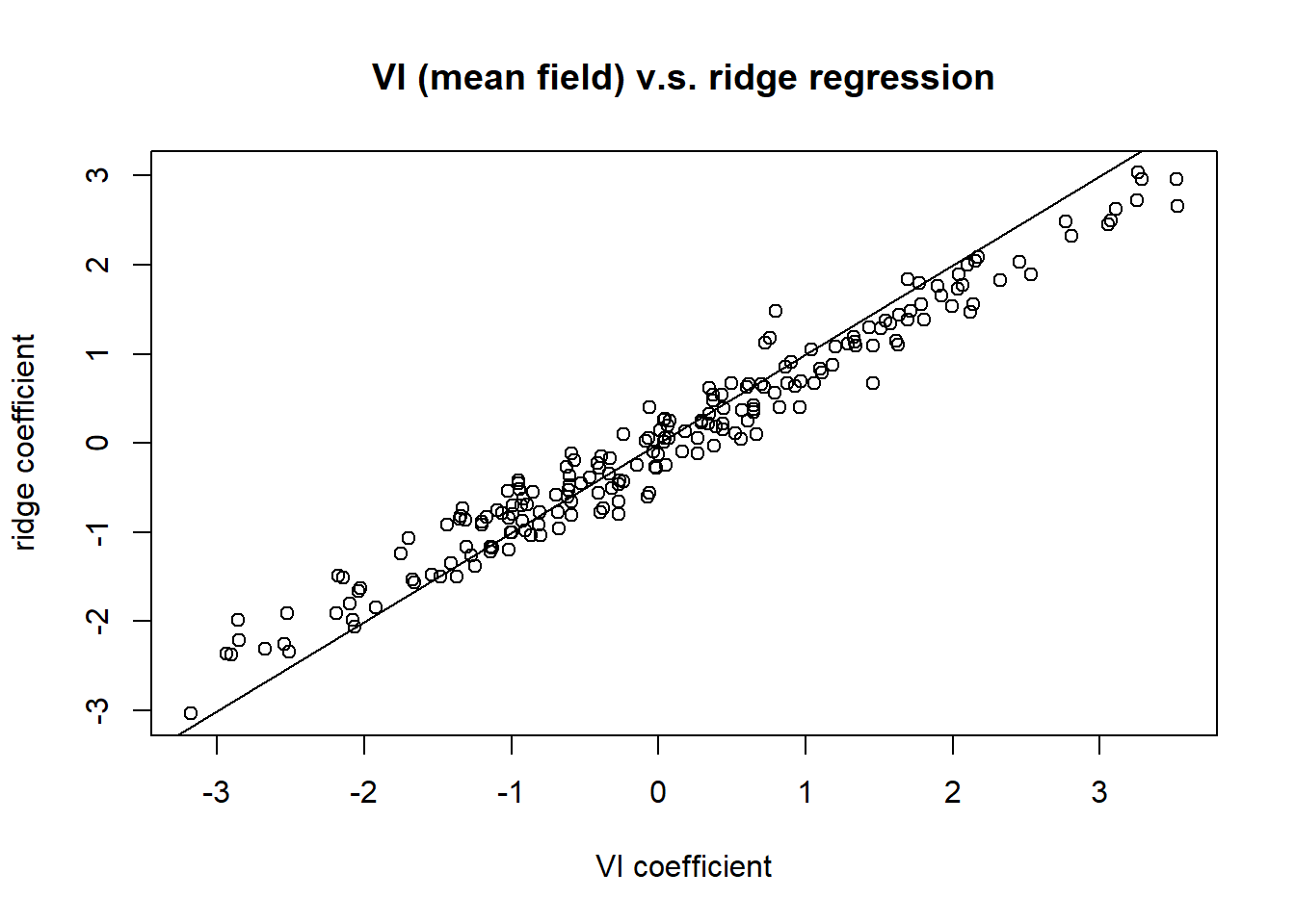
| Version | Author | Date |
|---|---|---|
| 38b5b82 | Zhengyang Fang | 2019-06-27 |
[1] TRUEThe VI algorithm converges, and those two results agree well, which justifies our algorithm.
A notable fact is that, all elements in \(\textbf X\) are independently generated, thus the columns of \(\textbf X\) are independent. When the sample size is large, those columns should be approximately orthogonal to each other. This matches the assumption of mean field method. This is an important reason for why their results agree well.
III. Performance for special \(\textbf X\)
We test mean field method for the two following extreme cases.
- Columns of \(\textbf X\) are orthogonal, which perfectly matches the assumption of mean field method.
library(pracma)

# use Gram-Schmidt orthogonalized X, s.t. its columns are orthogonal
col_ortho.X <- gramSchmidt(X)$Q * sqrt(n)
col_ortho.Y <- rnorm (n, col_ortho.X %*% true.beta + 1, sigma)

compare(col_ortho.X, col_ortho.Y, plot.title = "Columns of X are orthogonal")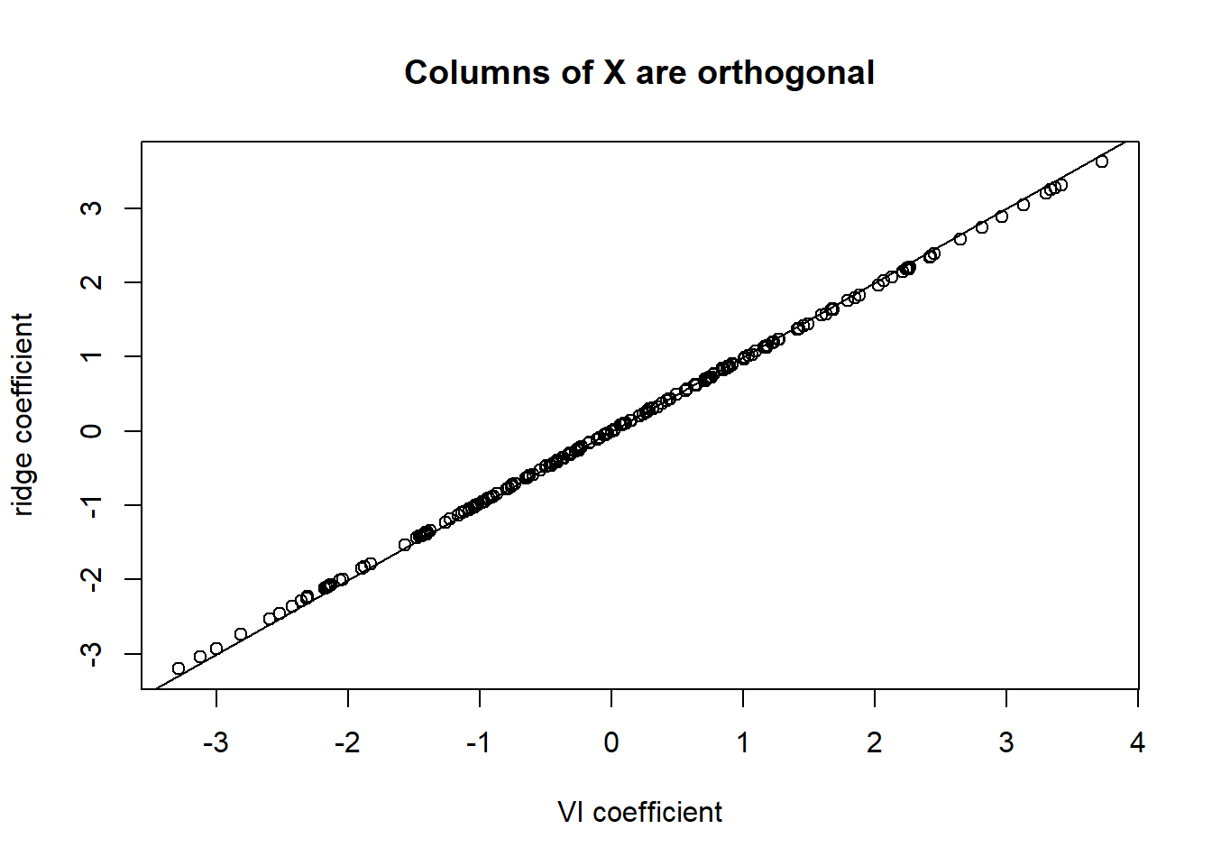
[1] TRUETheir results match perfectly well. In this case, mean field method approximation is the exact solution (up to the convergence precision).
- Columns of \(\textbf X\) are highly correlated, which violates the assumption of mean field method.
In this simulation, we first let all columns of \(\textbf X\) to be exactly the same, and then add a small Gaussian perturbation on each term. So that all columns are highly correlated.
col_rep.X <- matrix(X[, 1], nrow = n, ncol = p) +
             matrix(rnorm(n * p, sd = 0.1), nrow = n, ncol = p)
col_rep.Y <- rnorm (n, col_rep.X %*% true.beta + 1, sigma)

compare(col_rep.X, col_rep.Y, plot.title = "Columns of X are highly correlated")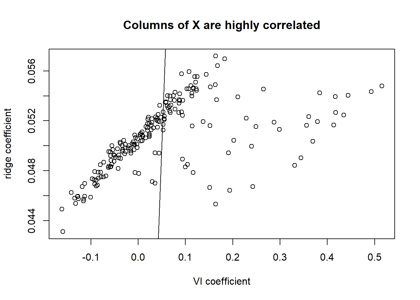
| Version | Author | Date |
|---|---|---|
| 38b5b82 | Zhengyang Fang | 2019-06-27 |
[1] FALSEFrom the plot we can see that, mean field method approximation can be terrible, as the assumption of mean field method is violated.
sessionInfo()R version 3.6.0 (2019-04-26)
Platform: x86_64-w64-mingw32/x64 (64-bit)
Running under: Windows 10 x64 (build 17134)
Matrix products: default
locale:
[1] LC_COLLATE=English_United States.1252
[2] LC_CTYPE=English_United States.1252
[3] LC_MONETARY=English_United States.1252
[4] LC_NUMERIC=C
[5] LC_TIME=English_United States.1252
attached base packages:
[1] stats graphics grDevices utils datasets methods base
other attached packages:
[1] pracma_2.2.5 glmnet_2.0-18 foreach_1.4.4 Matrix_1.2-17 MASS_7.3-51.4
[6] lasso2_1.2-20
loaded via a namespace (and not attached):
[1] Rcpp_1.0.1 knitr_1.23 whisker_0.3-2 magrittr_1.5
[5] workflowr_1.4.0 lattice_0.20-38 stringr_1.4.0 tools_3.6.0
[9] grid_3.6.0 xfun_0.7 git2r_0.25.2 htmltools_0.3.6
[13] iterators_1.0.10 yaml_2.2.0 rprojroot_1.3-2 digest_0.6.19
[17] fs_1.3.1 codetools_0.2-16 glue_1.3.1 evaluate_0.14
[21] rmarkdown_1.13 stringi_1.4.3 compiler_3.6.0 backports_1.1.4