Ridge regression with algorithm in [Carbonetto and Stephens, 2012]
Zhengyang Fang
June 27, 2019
Last updated: 2019-08-01
Checks: 7 0
Knit directory: susie-mixture/analysis/
This reproducible R Markdown analysis was created with workflowr (version 1.4.0). The Checks tab describes the reproducibility checks that were applied when the results were created. The Past versions tab lists the development history.
Great! Since the R Markdown file has been committed to the Git repository, you know the exact version of the code that produced these results.
Great job! The global environment was empty. Objects defined in the global environment can affect the analysis in your R Markdown file in unknown ways. For reproduciblity it’s best to always run the code in an empty environment.
The command set.seed(1) was run prior to running the code in the R Markdown file. Setting a seed ensures that any results that rely on randomness, e.g. subsampling or permutations, are reproducible.
Great job! Recording the operating system, R version, and package versions is critical for reproducibility.
Nice! There were no cached chunks for this analysis, so you can be confident that you successfully produced the results during this run.
Great job! Using relative paths to the files within your workflowr project makes it easier to run your code on other machines.
Great! You are using Git for version control. Tracking code development and connecting the code version to the results is critical for reproducibility. The version displayed above was the version of the Git repository at the time these results were generated.
Note that you need to be careful to ensure that all relevant files for the analysis have been committed to Git prior to generating the results (you can use wflow_publish or wflow_git_commit). workflowr only checks the R Markdown file, but you know if there are other scripts or data files that it depends on. Below is the status of the Git repository when the results were generated:
Ignored files:
    Ignored:    .RData
    Ignored:    .Rhistory
    Ignored:    .Rproj.user/
    Ignored:    analysis/.RData
    Ignored:    analysis/.Rhistory
Note that any generated files, e.g. HTML, png, CSS, etc., are not included in this status report because it is ok for generated content to have uncommitted changes.
These are the previous versions of the R Markdown and HTML files. If you’ve configured a remote Git repository (see ?wflow_git_remote), click on the hyperlinks in the table below to view them.
| File | Version | Author | Date | Message |
|---|---|---|---|---|
| html | 034283b | Zhengyang Fang | 2019-07-22 | Build site. |
| html | 6d9cbaa | Zhengyang Fang | 2019-07-22 | Build site. |
| html | 2a474f9 | Zhengyang Fang | 2019-07-22 | Build site. |
| Rmd | dfb3b4c | Zhengyang Fang | 2019-07-22 | wflow_publish(dir()) |
| html | c72a707 | Zhengyang Fang | 2019-07-22 | Build site. |
| html | 8092e5a | Zhengyang Fang | 2019-07-19 | Build site. |
| html | 5d3e3ef | Zhengyang Fang | 2019-07-11 | Build site. |
| html | 3eee187 | Zhengyang Fang | 2019-07-03 | Build site. |
| html | f303e14 | Zhengyang Fang | 2019-07-01 | Build site. |
| html | def2b27 | Zhengyang Fang | 2019-06-28 | Build site. |
| html | 05f778b | Zhengyang Fang | 2019-06-28 | Build site. |
| html | 7e8adc5 | Zhengyang Fang | 2019-06-27 | Build site. |
| Rmd | d10e0d7 | Zhengyang Fang | 2019-06-27 | wflow_publish(“ridge_VI_carbo2012.Rmd”) |
| html | 16cad80 | Zhengyang Fang | 2019-06-27 | Build site. |
| Rmd | a60a6e8 | Zhengyang Fang | 2019-06-27 | wflow_publish(“ridge_VI_carbo2012.Rmd”) |
| html | 354e4b3 | Zhengyang Fang | 2019-06-27 | Build site. |
| Rmd | f209966 | Zhengyang Fang | 2019-06-27 | wflow_publish(“ridge_VI_carbo2012.Rmd”) |
A trivial application of the reference: ridge regression
Ridge regression is a special case for BVSR: the spike-and-slab prior degenerates to a slab Gaussian prior.
In this case we can fix \(\pi=1\), and ignore \(\gamma\), also the estimated PIP \(\alpha_k=1\) always holds.
We apply the same algorithm above to this simplified case. In step 2, we only have to update \(\mu_k\) in the coordinate descent step, and it will be much easier.
Also, we can simplify our problem from two following aspects.
I. Importance weight approximation
Also, the importance weight approximation in step 3 gets easier. We can solve it out, instead of estimating it.
Actually, the nasty part \(\mathbb P(y|\textbf X,\theta)\) can be calculated by the following integration
\[ \mathbb P(y|\textbf X,\theta)=\int \mathbb P(y|\textbf X,\theta,\beta)p(\beta)d\beta. \]
Where \(p(\beta)\) is the prior of \(\beta\): \[ \beta|\sigma_\beta\sim N(0,\sigma^2_b\sigma^2). \]
For the likelihood term, we have \[ \hat\beta\sim N\left(\beta,(\textbf X^T\textbf X)^{-1}\sigma^2\right), \] where \[ \hat\beta=(\textbf X^T\textbf X)^{-1}\textbf X^TY. \]
Since the prior and likelihood are both Gaussian, the posterior distribution of \(\beta\) should also be Gaussian. Thus
\[ \begin{aligned} \int \mathbb P(y|\textbf X,\theta,\beta)p(\beta)d\beta &=(2\pi)^{-p}\sigma^{-2}|\textbf X^T\textbf X|^{1/2}\sigma_{\beta}^{-1} \int \exp\left\{-\frac1{2\sigma^2}\left({(\beta-\hat\beta)^T(\textbf X^T\textbf X)(\beta-\hat\beta)+\beta^T \beta/\sigma_\beta^2}\right)\right\}d\beta\\ &=\frac{C_0C_1}{C_2}\int \exp\left\{-\frac1{2\sigma^2}(\beta-\hat\beta_{ridge})^T\left(\textbf X^T\textbf X+\frac{\textbf I}{\sigma_b^2}\right)(\beta-\hat\beta_{ridge})\right\}d\beta\\ &=\frac{C_0C_1}{C_2C_3}, \end{aligned} \]
where \(\hat\beta=(\textbf X^T\textbf X)^{-1}\textbf X^T Y\), \(\hat\beta_{ridge}=(\textbf X^T\textbf X+\textbf I/\sigma^2_b)^{-1}\textbf X^T Y\), \(C_0=(2\pi)^{-p}\sigma^{-2}|\textbf X^T\textbf X|^{1/2}\sigma_b^{-1}\), \(C_1=\exp\left\{-\frac1{2\sigma^2}\hat\beta^T(\textbf X^T\textbf X)\hat\beta\right\}\), \(C_2=\exp\left\{-\frac1{2\sigma^2}\hat\beta_{ridge}^T(\textbf X^T\textbf X+\textbf I/\sigma_b^2)\hat\beta_{ridge}\right\}\), and \(C_3=(2\pi)^{-p/2}\sigma^{-1}\left|\textbf X^T\textbf X+\textbf I/\sigma_b^2\right|^{-1/2}\).
Finally we have
\[ \mathbb P(y|\textbf X,\theta)=\frac{|\textbf X^T\textbf X|^{1/2}\cdot|\textbf X^T\textbf X+\textbf I/\sigma_b^2|^{1/2}}{(2\pi)^{p/2}\sigma}\exp\left\{-\frac1{2\sigma^2}Y^T\textbf X\left((\textbf X^T\textbf X)^{-1}-(\textbf X^T\textbf X+\textbf I/\sigma^2_b)^{-1}\right)\textbf X^TY\right\}. \]
II. Choosing the prior of \(\theta\)
In the reference paper, we use \(p(\sigma^2)\propto \frac 1{\sigma^2}\) as the prior of \(\sigma^2\). The prior of \(\sigma_\beta^2\) is suggested in Guan and Stephens (2011).
For simplicity, we estimate \(\sigma_\beta^2\) by MLE, and fix it.
A notable fact is that, in the ridge regression setting, we solve optimization problem \[
\min_\beta \|Y-X\beta\|_2^2+\lambda\|\beta\|_2^2
\] for fixed penalty parameter \(\lambda\). It is equivalent to fix \(\sigma_\beta^2=\frac1\lambda\) in the Bayesian setting. However, according to the simulation result, they are not perfectly equal. It might be because the coordinate-descent algorithm does not converge to the global optimum.
III. Simulation
Algorithm code
#' VI.ridge: use variational inference in ridge regression
#' @param X: variables in linear model
#' @param Y: response in linear model
#' @param N: the number of importance sampling
#' @return the estimated beta, result of ridge regression

VI.ridge <- function (X, Y, sigma.b, N = 50) {
    prior <- function (sigma2) {
        return (1 / sigma2)
    }

    p <- ncol(X)
    n <- nrow(X)

    # intercept
    beta.hat <- numeric(p + 1)
    beta.hat[1] <- mean(Y)

    # center the columns of X and Y
    Y <- Y - mean(Y)
    X <- t(t(X) - colMeans(X))

    # preprocess to make it faster
    XtX <- t(X) %*% X
    Xy  <- t(X) %*% Y

    Z.exp <- t(Xy) %*% (solve(XtX) - solve(XtX + diag(p) / (sigma.b ^ 2))) %*% Xy
    # Z \propto 1/sigma * exp(-Z.exp / 2sigma^2)

    sigma2 <- runif (N, min = 0, max = 10)
    weight <- prior(sigma2)
    s      <- numeric(p)

    mu     <- matrix(0, nrow = N, ncol = p) # each row is a sample

    for (i in 1: N) {
        s2 <- sigma2[i] / (diag(XtX) + 1 / (sigma.b ^ 2))
        converge <- FALSE
        iter <- 0
        while (!converge && iter < 50) {
            converge = TRUE
            iter <- iter + 1

            for (k in 1: p) {
                record <- mu[i, k]

                mu[i, k] <- s2[k] / sigma2[i] *
                            (Xy[k] - mu[i, ] %*% XtX[, k]  + XtX[k, k] * mu[i, k])

                if (abs(mu[i, k] - record) > 1e-4)
                    converge <- FALSE
            }
        }

        Z <- exp(-Z.exp / (2 * sigma2[i])) / sqrt(sigma2[i])
        weight[i] <- Z * weight[i]
    }

    # take the weighted average of the sampled posterior mean
    weight <- weight / sum(weight)
    beta.hat[2: (p + 1)] <- t(mu) %*% weight

    result <- list()
    result$coef <- beta.hat
    result$weight <- weight
    result$mu <- mu

    return (result)
}
#VI.coef <- VI.ridge(X, Y, sqrt(1 / lambda))
Generate data with \(\textbf X\in\mathbb R^{50\times30}\).
set.seed(1)

# generate data
sigma   <- 3
sigma.b <- 0.5
p       <- 200
n       <- 300

true.beta <- rnorm (p, 0, sd = sigma.b * sigma)
X <- matrix (rnorm (n * p), nrow = n, ncol = p)
Y <- rnorm (n, X %*% true.beta + 1, sigma)
Compared with ridge regression, where the tuning parameter in ridge regression is chosen by cross-validation:
library(lasso2)
library(MASS)
library(glmnet)

cvfit <- cv.glmnet(X, Y, alpha = 0)
lambda <- cvfit$lambda.1se
# remove the intercept
ridge.coef <- coef(cvfit, s = "lambda.1se")[2: (p + 1)]

VI.result <- VI.ridge(X, Y, sqrt(1 / lambda))
# remove the intercept
VI.coef   <- VI.result$coef[2: (p + 1)]

plot (VI.coef, ridge.coef, main = 'VI v.s. ridge regression',
      xlab = 'VI coefficient', ylab = 'ridge coefficient')
abline(a = 0, b = 1)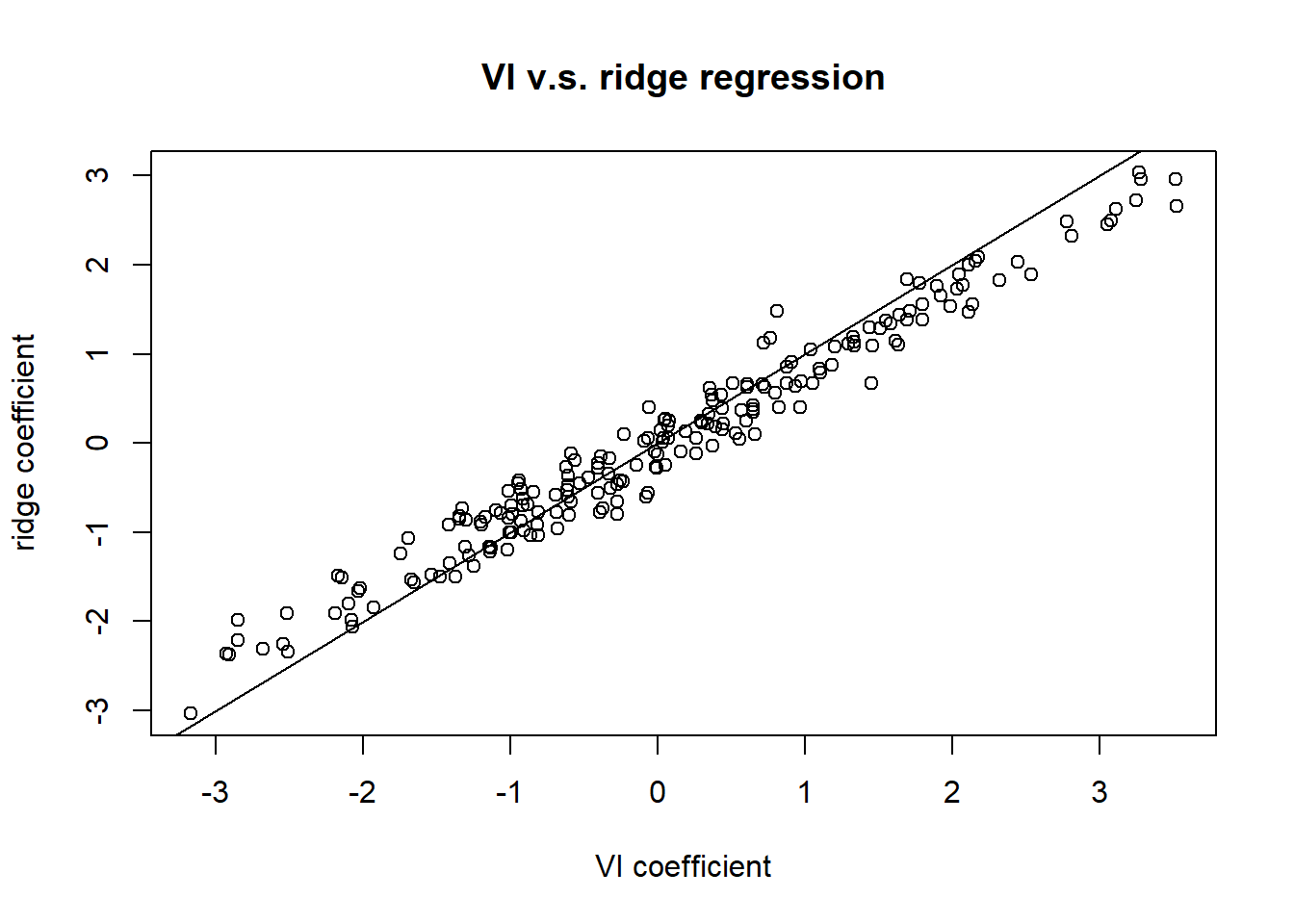
| Version | Author | Date |
|---|---|---|
| 354e4b3 | Zhengyang Fang | 2019-06-27 |
The VI result and the ridge regression result are close to each other. As ridge regression finds the exact posterior estimate, VI returns a reasonable approximation.
sessionInfo()R version 3.6.0 (2019-04-26)
Platform: x86_64-w64-mingw32/x64 (64-bit)
Running under: Windows 10 x64 (build 17134)
Matrix products: default
locale:
[1] LC_COLLATE=English_United States.1252
[2] LC_CTYPE=English_United States.1252
[3] LC_MONETARY=English_United States.1252
[4] LC_NUMERIC=C
[5] LC_TIME=English_United States.1252
attached base packages:
[1] stats graphics grDevices utils datasets methods base
other attached packages:
[1] glmnet_2.0-18 foreach_1.4.4 Matrix_1.2-17 MASS_7.3-51.4 lasso2_1.2-20
loaded via a namespace (and not attached):
[1] Rcpp_1.0.1 knitr_1.23 whisker_0.3-2 magrittr_1.5
[5] workflowr_1.4.0 lattice_0.20-38 stringr_1.4.0 tools_3.6.0
[9] grid_3.6.0 xfun_0.7 git2r_0.25.2 htmltools_0.3.6
[13] iterators_1.0.10 yaml_2.2.0 rprojroot_1.3-2 digest_0.6.19
[17] fs_1.3.1 codetools_0.2-16 glue_1.3.1 evaluate_0.14
[21] rmarkdown_1.13 stringi_1.4.3 compiler_3.6.0 backports_1.1.4