Experiment 2
Zhengyang Fang
July 12, 2019
Last updated: 2019-08-01
Checks: 6 1
Knit directory: susie-mixture/analysis/
This reproducible R Markdown analysis was created with workflowr (version 1.4.0). The Checks tab describes the reproducibility checks that were applied when the results were created. The Past versions tab lists the development history.
The R Markdown file has unstaged changes. To know which version of the R Markdown file created these results, you’ll want to first commit it to the Git repo. If you’re still working on the analysis, you can ignore this warning. When you’re finished, you can run wflow_publish to commit the R Markdown file and build the HTML.
Great job! The global environment was empty. Objects defined in the global environment can affect the analysis in your R Markdown file in unknown ways. For reproduciblity it’s best to always run the code in an empty environment.
The command set.seed(1) was run prior to running the code in the R Markdown file. Setting a seed ensures that any results that rely on randomness, e.g. subsampling or permutations, are reproducible.
Great job! Recording the operating system, R version, and package versions is critical for reproducibility.
Nice! There were no cached chunks for this analysis, so you can be confident that you successfully produced the results during this run.
Great job! Using relative paths to the files within your workflowr project makes it easier to run your code on other machines.
Great! You are using Git for version control. Tracking code development and connecting the code version to the results is critical for reproducibility. The version displayed above was the version of the Git repository at the time these results were generated.
Note that you need to be careful to ensure that all relevant files for the analysis have been committed to Git prior to generating the results (you can use wflow_publish or wflow_git_commit). workflowr only checks the R Markdown file, but you know if there are other scripts or data files that it depends on. Below is the status of the Git repository when the results were generated:
Ignored files:
    Ignored:    .RData
    Ignored:    .Rhistory
    Ignored:    .Rproj.user/
    Ignored:    analysis/.RData
    Ignored:    analysis/.Rhistory
    Ignored:    docs/presentation_files/

Unstaged changes:
    Deleted:    analysis/R_function/ridge.R
    Modified:   analysis/derivation_in_susie_mixture.Rmd
    Modified:   analysis/experiment2.Rmd
Note that any generated files, e.g. HTML, png, CSS, etc., are not included in this status report because it is ok for generated content to have uncommitted changes.
These are the previous versions of the R Markdown and HTML files. If you’ve configured a remote Git repository (see ?wflow_git_remote), click on the hyperlinks in the table below to view them.
| File | Version | Author | Date | Message |
|---|---|---|---|---|
| html | 2bbbe99 | Zhengyang Fang | 2019-08-01 | Build site. |
| Rmd | 746720f | Zhengyang Fang | 2019-08-01 | wflow_publish(dir()) |
| html | 034283b | Zhengyang Fang | 2019-07-22 | Build site. |
| Rmd | a434845 | Zhengyang Fang | 2019-07-22 | wflow_publish(dir()) |
| html | 6d9cbaa | Zhengyang Fang | 2019-07-22 | Build site. |
| Rmd | 4cfac44 | Zhengyang Fang | 2019-07-22 | wflow_publish(dir()) |
| html | 2a474f9 | Zhengyang Fang | 2019-07-22 | Build site. |
| Rmd | dfb3b4c | Zhengyang Fang | 2019-07-22 | wflow_publish(dir()) |
| html | c72a707 | Zhengyang Fang | 2019-07-22 | Build site. |
| Rmd | 2c9220d | Zhengyang Fang | 2019-07-22 | wflow_publish(dir()) |
| html | 8092e5a | Zhengyang Fang | 2019-07-19 | Build site. |
| Rmd | 3893538 | Zhengyang Fang | 2019-07-19 | wflow_publish(dir()) |
I. Generate Data
# Small script to simulated data that models the an idealized
# genome-wide association study, in which all single nucleotide
# polymorphisms (SNPs) have alternative alleles at high frequencies in
# the population (>5%), and all SNPs contribute some (small) amount of
# variation to the quantitative trait. The SNPs are divided into two
# sets: those that contribute a very small amount of variation, and
# those that contribute a larger amount of variable (these are the
# "QTLs"---quantitative trait loci).
#
# Adjust the five parameters below (r, d, n, p, i) to control how the
# data are enerated.
#
# Peter Carbonetto
# University of Chicago
# January 23, 2017
#
# Diploid

# The minor alleles have additive influence on a specific trait (y).
# (certered)  X: number of minor alleles


#' @function Generate.data()
#' @param r: Proportion of variance in trait explained by SNPs.
#' @param d: Proportion of additive genetic variance due to QTLs.
#' @param n: Number of samples.
#' @param p: Number of markers (SNPs).
#' @param i: Indices of the QTLs ("causal variants").
#' @return: a list of data, with element X, y, beta1, beta2

Generate.data <- function (r = 0.6, d = 0.4, n = 400, p = 1000, i = c(27, 54)){
    # GENERATE DATA SET
    # -----------------
    # Generate the minor allele frequencies. They are uniformly
    # distributed on [0.05,0.5].
    maf <- 0.05 + 0.45 * runif(p)

    # Simulate genotype data X from an idealized population according to the
    # minor allele frequencies generated above.
    X <- (runif(n*p) < maf) +
         (runif(n*p) < maf)
    X <- matrix(as.double(X), n, p, byrow = TRUE)

    # Center the columns of X.
    rep.row <- function (x, n)
      matrix(x, n, length(x), byrow = TRUE)
    X <- X - rep.row(colMeans(X), n)

    # Generate (small) polygenic additive effects for the SNPs.
    u <- rnorm(p)

    # Generate (large) QTL effects for the SNPs.
    beta    <- rep(0, p)
    beta[i] <- rnorm(length(i))

    # Adjust the additive effects so that we control for the proportion of
    # additive genetic variance that is due to QTL effects (d) and the
    # total proportion of variance explained (r). That is, we adjust beta
    # and u so that
    #
    #   r = a/(a+1)
    #   d = b/a,
    #
    # where I've defined
    #
    #   a = (u + beta)'*cov(X)*(u + beta),
    #   b = beta'*cov(X)*beta.
    #
    # Note: this code only works if d or r are not exactly 0 or exactly 1.
    st   <- c(r/(1-r) * d / var(X %*% beta))
    beta <- sqrt(st) * beta
    sa   <- max(Re(polyroot(c(c(var(X %*% beta) - r/(1-r)),
                              2*sum((X %*% beta) * (X %*% u))/n,
                              c(var(X %*% u))))))^2
    u    <- sqrt(sa) * u

    # Generate the quantitative trait measurements.
    y <- c(X %*% (u + beta) + rnorm(n, sd = 0.1))

    data <- list()
    data$X     <- X
    data$y     <- y
    data$beta1 <- u
    data$beta2 <- beta
    data$s1    <- sa
    data$s2    <- st

    return (data)
}
# Initialize random number generation so that the results are reproducible.
set.seed(1)

r <- 0.3
d <- 0.7
n <- 50
p <- 100
idx <- c(1, 2)

data <- Generate.data(r, d, n, p, idx)
X <- data$X
y <- data$y
II. Example
Due to the numerical issues in optimizing the log-likelihood, I use a small data set where \(n=100,p=200\).
# initialize susie object s
# so that we can run update_each_effect()

init <- function (n, p, L) {
    s <- list()
    s$alpha  <- matrix(0, nrow = L, ncol = p)
    s$Xr     <- rep(0, n)
    s$mu     <- matrix(0, nrow = L, ncol = p)
    s$mu2    <- matrix(0, nrow = L, ncol = p)
    s$sigma2 <- 1
    s$pi     <- rep(1 / p, p)
    s$V      <- rep(1, L)
    s$converge <- FALSE

    class(s) <- "susie"

    return (s)
}

ridge.elbo <- function(beta.hat, X, r, res, sigma2, sigma.b2) {
    n <- nrow(X)
    p <- ncol(X)

    llh <- loglikelihood(sigma.b2, X, r, sigma2)

    return (llh + n / 2 * log (2 * pi * sigma2) + sum(res ^ 2) / (2 * sigma2))
}

ridge <- function (X, y, sigma.b2, sigma2) {
    n <- nrow(X)
    p <- ncol(X)

    S.inv <- solve(crossprod(X) + (sigma2 / sigma.b2) * diag(p))
    beta.hat <- S.inv %*% t(X) %*% y
    beta.var <- sigma2 * crossprod(X %*% S.inv)

    result <- list()
    result$beta.hat <- beta.hat
    result$var      <- beta.var

    return (result)
}

loglikelihood <- function (sigma.b2, X, y, sigma2) {
    XtX <- crossprod(X)
    Xty <- crossprod(X, y)

    p <- nrow(XtX)
    n <- nrow(X)

    S <- XtX + (sigma2 / sigma.b2) * diag(p)

    term1 <- t(Xty) %*% solve(S) %*% Xty / sigma2 - n * log(2 * pi)

    # sum(log(eigen(S)$values)): log(det(S))
    term2 <- - sum(log(eigen(S)$values))

    term3 <- - n * log (sigma2) - sum(y ^ 2) / sigma2 - p * log(sigma.b2)

    return ((term1 + term2 + term3) / 2)
}

ELBO.equation <- function (log.sigma.b, XtX, Xty, sigma2) {
    sigma.b2 <- exp(2 * log.sigma.b)

    p <- ncol(XtX)
    S.inv <- solve(sigma.b2 * XtX + sigma2 * diag(p))

    u <- S.inv %*% Xty

    return (sum(u ^ 2) - p)
}

MLE <- function (X, y, sigma2) {
    XtX <- crossprod(X)
    Xty <- crossprod(X, y)

    log.sigma.b <- uniroot(ELBO.equation, interval = c(-6, 6),
                           XtX = XtX, Xty = Xty, sigma2 = sigma2)$root

    return (exp(log.sigma.b * 2))
}
#'Susie mixture function
#' @param X: An n by p matrix covariates
#' @param Y: A vectore of length n response
#' @param L: Number of components
#' @param verbose: Keep track of the ELBO and print it to the console
susie.mixture <- function(X, Y, L, tol = 0.001, max_iter = 100, intercept = TRUE,
coverage = 0.95, min_abs_corr = 0.5, verbose = F) {
p = ncol(X)
n = nrow(X)
s <- init(n, p, L)
elbo <- rep(0, max_iter)
ridge.bar <- rep(0, p)
if (intercept) {
mean_y <- mean(Y)
Y <- Y - mean_y
}
for(i in 1: max_iter){
# susie update
s <- update_each_effect(X, Y, s)
if(verbose){
obj <- get_objective(X, Y, s)
if (i > 1) {
obj <- obj + ridge.elbo(ridge.bar, X, r, ridge.res, s$sigma2, sigma.b2)
print(paste0("objective (after susie update):", obj))
}
}
# ridge regression update
Y <- Y + X %*% ridge.bar
r <- Y - s$Xr
# find the optimal prior variance by maximizing the ELBO
sigma.b2 <- MLE(X, r, s$sigma2)
ridge.fit <- ridge(X, r, sigma.b2, s$sigma2)
ridge.bar <- ridge.fit$beta.hat
ridge.var <- diag(X %*% ridge.fit$var %*% t(X))
Y <- Y - X %*% ridge.bar
ridge.res <- r - X %*% ridge.bar
if(verbose){
print (mean(r^2))
print(paste0("sigma.b^2:", sigma.b2))
obj <- get_objective(X, Y, s) +
ridge.elbo(ridge.bar, X, r, ridge.res, s$sigma2, sigma.b2)
print(paste0("objective (after ridge update):", obj))
}
s$sigma2 = estimate_residual_variance(X, Y, s) + mean(ridge.var)
obj <- get_objective(X, Y, s) +
ridge.elbo(ridge.bar, X, r, ridge.res, s$sigma2, sigma.b2)
if(verbose)
print(paste0("objective (after update sigma2):", obj))
elbo[i + 1] <- obj
if((elbo[i + 1] - elbo[i]) < tol) {
s$converged <- TRUE
break;
}
}
elbo <- elbo[2: (i + 1)] # Remove first (infinite) entry, and trailing NAs.
s$elbo <- elbo
s$niter <- i
if (is.null(s$converged)) {
warning(paste("IBSS algorithm did not converge in", max_iter, "iterations!"))
s$converged = FALSE
}
if(intercept){
s$intercept = mean_y - sum(attr(X,"scaled:center") * (colSums(s$alpha*s$mu)/attr(X,"scaled:scale")))# estimate intercept (unshrunk)
s$fitted = s$Xr + mean_y
} else {
s$intercept <- 0
s$fitted <- s$Xr
}
s$fitted <- drop(s$fitted)
## SuSiE PIP
s$null_index = 0
s$pip = susie_get_pip(s)
## mixture
s$sigma.b2 <- sigma.b2
s$ridge.coef <- ridge.fit$beta.hat
return(s)
}
library(R.utils)
sourceDirectory("R_function")
s <- susie(X, y, L = 2, verbose = T, scaled_prior_variance = 0.5,
estimate_prior_variance = FALSE, standardize = FALSE) [1] "objective:-44.5319038772319"
[1] "objective:-38.7993191041671"
[1] "objective:-36.2925884480723"
[1] "objective:-34.9486493391848"
[1] "objective:-34.647911036539"
[1] "objective:-34.6204326163046"
[1] "objective:-34.6177278158765"
[1] "objective:-34.617616355774"
[1] "objective:-34.6176066780397"
[1] "objective:-34.6176062968079"sm <- susie.mixture(X, y, L = 2, verbose = T)[1] 0.3978632
[1] "sigma.b^2:0.0438337538720929"
[1] "objective (after ridge update):-76.5966437053549"
[1] "objective (after update sigma2):-32.784976098098"par(mfrow = c(2, 2))
plot(susie_get_pip(sm), abs(data$beta1 + data$beta2),
main = "SuSiE mixture", xlab = "PIP", ylab = "Random effect + Fixed effect")
plot(susie_get_pip(sm), abs(data$beta2),
main = "SuSiE mixture", xlab = "PIP", ylab = "Only fixed effect")
plot(susie_get_pip(s), abs(data$beta1 + data$beta2),
main = "SuSiE", xlab = "PIP", ylab = "Random effect + Fixed effect")
plot(susie_get_pip(s), abs(data$beta2),
main = "SuSiE", xlab = "PIP", ylab = "Only fixed effect")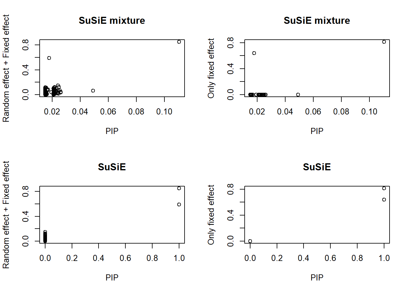
| Version | Author | Date |
|---|---|---|
| 2bbbe99 | Zhengyang Fang | 2019-08-01 |
As expected, SuSiE-mixture model shrinks the PIP, and makes less discovery.
III. Important details in the coding
- The order of the
ridge regressionstep and thesusiestep
In the experiment, if I do the ridge regression step first and then the susie step, then the ridge regression takes charge of most of the signal in the data set, and leaving barely nothing for the susie step to find. It causes failure to converge. Therefore, I do the ridge regression step after the susie step.
- Update \(\sigma_b^2\) by maximizing
ELBO
In the ridge regression step, the ELBO can be written as
\[ \begin{aligned} ELBO(q_0)=&\mathbb E_{q_0}\log p(X,\bar r_0;\beta)-\mathbb E_{q_0}\log q_0(\beta)\\ =&\mathbb E_{q_0} \left[\log (N(\bar r_0;X\beta,\sigma^2 I)\cdot N(\beta;0,\sigma_b^2I))-\log q_0(\beta)\right]\\ =&\mathbb E_{q_0} \left[\log\left( \frac{\exp\left\{(\hat{\beta}_{ridge}^TX^T\bar r_0-\|\bar r_0\|^2_2)/(2\sigma^2)\right\}}{\sigma^n\sigma^p_b}\cdot N(\beta;\hat\beta_{ridge},\hat\Sigma)\right)-\log q_0(\beta)\right]+const\\ =&(\hat{\beta}_{ridge}^TX^T\bar r_0-\|\bar r_0\|^2_2)/(2\sigma^2)-n\log\sigma-p\log\sigma_b-KL(q_0||N(\hat\beta_{ridge},\Sigma_{ridge}))+const\\ \geq &(\hat{\beta}_{ridge}^TX^T\bar r_0-\|\bar r_0\|^2_2)/(2\sigma^2)-n\log\sigma-p\log\sigma_b+const:=G\\ \end{aligned} \]
The equality holds when \(q_0(\beta)\) is exactly \(N(\hat\beta_{ridge},\Sigma_{ridge})\).
Let
\[ \frac{\partial G}{\partial \sigma_b}=\frac1{2\sigma^2}(\bar r_0^TX S^{-1}(\frac{2\sigma^2}{\sigma_b^3})S^{-1} X^T\bar r_0)-\frac p{\sigma_b}=0. \]
Thus
\[ \|(\sigma_b^2X^TX+\sigma^2I)^{-1}X^T\bar r_0\|_2^2=p. \]
We can solve this with uniroot() function.
- The calculation of
ELBO
In susie algorithm, ELBO is the convergence criterion. So computing the ELBO is required. Follow the notation of the additive effects model (in appendix B.2 of the SuSiE paper), let \(\mu_0=X\beta_0\), where \(\beta_0\) is the coefficients in ridge regression step.
Then basically we use
\[ \begin{aligned} ELBO:=&F(q,g,\sigma^2;y)=-\frac n2\log(2\pi\sigma^2)-\frac1{2\sigma^2}\mathbb E_q\|y-\sum_{l=0}^L\mu_l\|_2^2+\sum_{l=0}^L\mathbb E_{q_l}\log\frac{g_l(\mu_l)}{q_l(\mu_l)}\\ =&-\frac n2\log(2\pi\sigma^2)-\frac1{2\sigma^2}\mathbb E_q\|y-\mu_0-\sum_{l=1}^L\mu_l\|_2^2+\mathbb E_{q_0}\log\frac{g_0(\mu_0)}{q_0(\mu_0)}+\sum_{l=1}^L\mathbb E_{q_l}\log\frac{g_l(\mu_l)}{q_l(\mu_l)}\\ =&\left(-\frac n2\log(2\pi\sigma^2)-\frac1{2\sigma^2}\mathbb E_q\|(y-\bar\mu_0)-\sum_{l=1}^L\mu_l\|_2^2+\sum_{l=1}^L\mathbb E_{q_l}\log\frac{g_l(\mu_l)}{q_l(\mu_l)}\right)-\frac1{2\sigma^2}\sum_{i=1}^nVar(\mu_{0i})+E_{q_0}\log\frac{g_0(\mu_0)}{q_0(\mu_0)}\\ \end{aligned} \]
The first term in the bracket is the ELBO for original susie, it can be computed by the built-in function get_objective(), with \(Y=y-\hat\mu_0\).
Let \(\sigma^2_b\) be the MLE of the prior variance of coefficients in ridge regression, and \(S=X^TX+\frac{\sigma^2}{\sigma^2_b}I\), we have \(\beta_{ridge}\sim N(S^{-1}X^Ty,S^{-1}X^TXS^{-1}\sigma^2)\). Also we have \(\mu_0=X\beta_{ridge}\), Thus \(\hat\mu_0=XS^{-1}X^Ty\), and \(\sum_{i=1}^nVar(\mu_{0i})=tr(\sigma^2XS^{-1}X^TXS^{-1}X^T)\). We can use those to compute the first two terms in ELBO.
As for the last term \(E_{q_0}\log\frac{g_0(\mu_0)}{q_0(\mu_0)}\), we use equation (B.15) in the susie paper
\[ \mathbb E_{q_l}\log\frac{g_l(\mu_l)}{q_l(\mu_l)}=\log l_l(\bar r;g_l,\sigma^2)+\frac n2\log(2\pi\sigma^2)+\frac1{2\sigma^2}\mathbb E_{q_l}\|\bar r_l-\mu_l\|^2_2. \]
For ridge regression \(l=0\), the first term is simply the log-likelihood, the second term is known, and the third term is \(\frac1{2\sigma^2}(\|\bar r_0-X\beta_{ridge}\|^2_2+\sum_{i=1}^nVar(\mu_{0i}))\). We can calculate them with the result above.
- Updating \(\sigma^2\)
We use
\[ \sigma^2=\frac{ERSS(y,\bar\mu,\bar{\mu^2})}{n}=\frac{\|(y-\bar\mu_0)-\sum_{l=1}^L\bar\mu_l\|^2_2+\sum_{l=1}^L\sum_{i=1}^nVar(\mu_{li})+\sum_{i=1}^nVar(\mu_{0i})}{n} \]
to update \(\sigma^2\). That is, we calculate the ERSS with the built-in function estimate_residual_variance() in original susie, with \(Y=y-\bar\mu_0\). Then it will take care of the first two terms. Now all we need to do is add an additional term \(\frac{\sum_{i=1}^nVar(\mu_{0i})}{n}\) to the returned value of estimate_residual_variance(). The value of \(\sum_{i=1}^nVar(\mu_{0i})\) is showed in bullet 3 above.
sessionInfo()R version 3.6.0 (2019-04-26)
Platform: x86_64-w64-mingw32/x64 (64-bit)
Running under: Windows 10 x64 (build 17134)
Matrix products: default
locale:
[1] LC_COLLATE=English_United States.1252
[2] LC_CTYPE=English_United States.1252
[3] LC_MONETARY=English_United States.1252
[4] LC_NUMERIC=C
[5] LC_TIME=English_United States.1252
attached base packages:
[1] stats graphics grDevices utils datasets methods base
other attached packages:
[1] R.utils_2.9.0 R.oo_1.22.0 R.methodsS3_1.7.1
loaded via a namespace (and not attached):
[1] workflowr_1.4.0 Rcpp_1.0.1 lattice_0.20-38 digest_0.6.19
[5] rprojroot_1.3-2 grid_3.6.0 backports_1.1.4 git2r_0.25.2
[9] magrittr_1.5 evaluate_0.14 stringi_1.4.3 fs_1.3.1
[13] whisker_0.3-2 Matrix_1.2-17 rmarkdown_1.13 tools_3.6.0
[17] stringr_1.4.0 glue_1.3.1 xfun_0.7 yaml_2.2.0
[21] compiler_3.6.0 htmltools_0.3.6 knitr_1.23