SuSiE-mixture Experiment 1
Zhengyang Fang
July 9, 2019
Last updated: 2019-08-01
Checks: 7 0
Knit directory: susie-mixture/analysis/
This reproducible R Markdown analysis was created with workflowr (version 1.4.0). The Checks tab describes the reproducibility checks that were applied when the results were created. The Past versions tab lists the development history.
Great! Since the R Markdown file has been committed to the Git repository, you know the exact version of the code that produced these results.
Great job! The global environment was empty. Objects defined in the global environment can affect the analysis in your R Markdown file in unknown ways. For reproduciblity it’s best to always run the code in an empty environment.
The command set.seed(1) was run prior to running the code in the R Markdown file. Setting a seed ensures that any results that rely on randomness, e.g. subsampling or permutations, are reproducible.
Great job! Recording the operating system, R version, and package versions is critical for reproducibility.
Nice! There were no cached chunks for this analysis, so you can be confident that you successfully produced the results during this run.
Great job! Using relative paths to the files within your workflowr project makes it easier to run your code on other machines.
Great! You are using Git for version control. Tracking code development and connecting the code version to the results is critical for reproducibility. The version displayed above was the version of the Git repository at the time these results were generated.
Note that you need to be careful to ensure that all relevant files for the analysis have been committed to Git prior to generating the results (you can use wflow_publish or wflow_git_commit). workflowr only checks the R Markdown file, but you know if there are other scripts or data files that it depends on. Below is the status of the Git repository when the results were generated:
Ignored files:
    Ignored:    .RData
    Ignored:    .Rhistory
    Ignored:    .Rproj.user/
    Ignored:    analysis/.RData
    Ignored:    analysis/.Rhistory
Note that any generated files, e.g. HTML, png, CSS, etc., are not included in this status report because it is ok for generated content to have uncommitted changes.
These are the previous versions of the R Markdown and HTML files. If you’ve configured a remote Git repository (see ?wflow_git_remote), click on the hyperlinks in the table below to view them.
| File | Version | Author | Date | Message |
|---|---|---|---|---|
| html | 034283b | Zhengyang Fang | 2019-07-22 | Build site. |
| html | 6d9cbaa | Zhengyang Fang | 2019-07-22 | Build site. |
| Rmd | 4cfac44 | Zhengyang Fang | 2019-07-22 | wflow_publish(dir()) |
| html | 2a474f9 | Zhengyang Fang | 2019-07-22 | Build site. |
| html | c72a707 | Zhengyang Fang | 2019-07-22 | Build site. |
| html | 8092e5a | Zhengyang Fang | 2019-07-19 | Build site. |
| Rmd | 3893538 | Zhengyang Fang | 2019-07-19 | wflow_publish(dir()) |
| html | 6a7d4d7 | Zhengyang Fang | 2019-07-12 | Build site. |
| Rmd | 7a47a30 | Zhengyang Fang | 2019-07-12 | wflow_publish(“experiment1.Rmd”) |
| html | 5d3e3ef | Zhengyang Fang | 2019-07-11 | Build site. |
| Rmd | 16c05dc | Zhengyang Fang | 2019-07-11 | wflow_publish(c(dir())) |
I. Generate Data
# Small script to simulated data that models the an idealized
# genome-wide association study, in which all single nucleotide
# polymorphisms (SNPs) have alternative alleles at high frequencies in
# the population (>5%), and all SNPs contribute some (small) amount of
# variation to the quantitative trait. The SNPs are divided into two
# sets: those that contribute a very small amount of variation, and
# those that contribute a larger amount of variable (these are the
# "QTLs"---quantitative trait loci).
#
# Adjust the five parameters below (r, d, n, p, i) to control how the
# data are enerated.
#
# Peter Carbonetto
# University of Chicago
# January 23, 2017
#
# Diploid

# The minor alleles have additive influence on a specific trait (y).
# (certered)  X: number of minor alleles


#' @function Generate.data()
#' @param r: Proportion of variance in trait explained by SNPs.
#' @param d: Proportion of additive genetic variance due to QTLs.
#' @param n: Number of samples.
#' @param p: Number of markers (SNPs).
#' @param i: Indices of the QTLs ("causal variants").
#' @return: a list of data, with element X, y, beta1, beta2

Generate.data <- function (r = 0.6, d = 0.4, n = 400, p = 1000, i = c(27,54,78)){
    # GENERATE DATA SET
    # -----------------
    # Generate the minor allele frequencies. They are uniformly
    # distributed on [0.05,0.5].
    maf <- 0.05 + 0.45 * runif(p)

    # Simulate genotype data X from an idealized population according to the
    # minor allele frequencies generated above.
    X <- (runif(n*p) < maf) +
         (runif(n*p) < maf)
    X <- matrix(as.double(X), n, p, byrow = TRUE)

    # Center the columns of X.
    rep.row <- function (x, n)
      matrix(x, n, length(x), byrow = TRUE)
    X <- X - rep.row(colMeans(X), n)

    # Generate (small) polygenic additive effects for the SNPs.
    u <- rnorm(p)

    # Generate (large) QTL effects for the SNPs.
    beta    <- rep(0, p)
    beta[i] <- rnorm(length(i))

    # Adjust the additive effects so that we control for the proportion of
    # additive genetic variance that is due to QTL effects (d) and the
    # total proportion of variance explained (r). That is, we adjust beta
    # and u so that
    #
    #   r = a/(a+1)
    #   d = b/a,
    #
    # where I've defined
    #
    #   a = (u + beta)'*cov(X)*(u + beta),
    #   b = beta'*cov(X)*beta.
    #
    # Note: this code only works if d or r are not exactly 0 or exactly 1.
    st   <- c(r/(1-r) * d / var(X %*% beta))
    beta <- sqrt(st) * beta
    sa   <- max(Re(polyroot(c(c(var(X %*% beta) - r/(1-r)),
                              2*sum((X %*% beta) * (X %*% u))/n,
                              c(var(X %*% u))))))^2
    u    <- sqrt(sa) * u

    # Generate the quantitative trait measurements.
    y <- c(X %*% (u + beta) + rnorm(n))

    data <- list()
    data$X     <- X
    data$y     <- y
    data$beta1 <- u
    data$beta2 <- beta
    data$s1    <- sa
    data$s2    <- st

    return (data)
}
# Initialize random number generation so that the results are
# reproducible.
set.seed(1)

r <- 0.6
d <- 0.4
n <- 400
p <- 1000
i <- c(27, 54, 78)

data <- Generate.data(r, d, n, p, i)
X <- data$X
y <- data$y
II. A simple intuitive sample
Compare the simulation result of SuSiE-mixture and SuSiE, with an arbitrarily chosen \(\sigma_1^2\).
library(susieR)

#' @function Susie.mixture: solve susie-mixture model with FIXED s1
#' @param X: the covariates of data
#' @param y: the response of data
#' @param s1: prior standard deviance of beta1
#' @return: a list, element `susie` is the result of susie on transformed data;
#'          element `beta1` is the result of ridge regression;
#'          element `beta2` is the estimated posterior mean of beta2

Susie.mixture <- function (X, y, s1) {
    K    <- tcrossprod(X)
    n    <- nrow(X)
    p    <- ncol(X)

    H    <- diag(n) + s1 * K
    L    <- t(tryCatch(chol(H), error = function(e) FALSE))
    Xhat <- solve(L, X)
    yhat <- solve(L, y)
    if (is.matrix(L))
        susie.result <- susie(X = Xhat, yhat, L = 10)

    beta2.hat <- colSums(susie.result$alpha * susie.result$mu)
    ridge.y   <- y - (X %*% beta2.hat)
    beta1.hat <- solve(crossprod(X) + s1 * diag(p), t(X) %*% ridge.y)

    ans <- list()
    ans$susie <- susie.result
    ans$beta1 <- beta1.hat
    ans$beta2 <- beta2.hat

    return (ans)
}

compare.result <- function (X, y, s1) {
    n  <- nrow(X)
    p  <- ncol(X)

    sm <- Susie.mixture (X, y, s1)
    beta2.hat <- sm$beta2

    # vanilla susie
    vanilla.result <- susie(X, y, L = 10)
    vanilla.beta2.hat <- colSums(vanilla.result$alpha * vanilla.result$mu)

    # Compare their PIP and posterior means

    par(mfrow = c(2, 2))
    plot(data$beta2, vanilla.beta2.hat, main = "SuSiE",
          xlab = "True coef", ylab = "posterior mean")
    plot(data$beta2, beta2.hat, main = "SuSiE-mixture",
          xlab = "True coef", ylab = "posterior mean")

    true.label    <- rep(FALSE, p)
    true.label[i] <- TRUE
    plot(true.label, vanilla.result$pip, main = "SuSiE",
          xlab = "True label", ylab = "PIP")
    plot(true.label, sm$susie$pip, main = "SuSiE-mixture",
          xlab = "True label", ylab = "PIP")
}


# The true s1 is around 0.05, different from the s1 used here
# But it still works well
compare.result(X, y, s1 = 1) 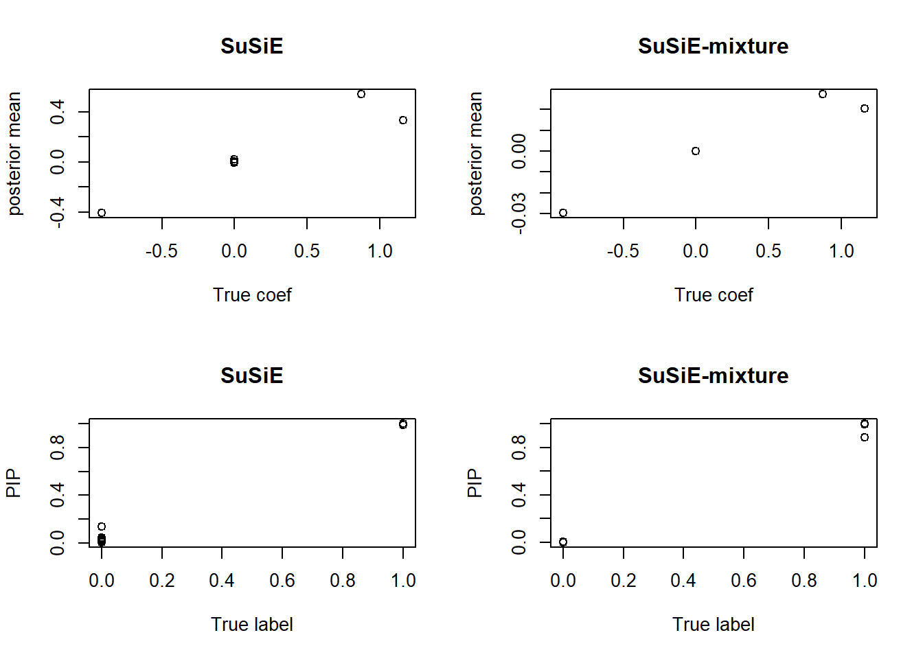
We plot the posterior mean of \(\hat\beta_2\) against the true coefficients \(\beta_2\), and plot the PIP against the true labels. Intuitively, SuSiE-mixture shrinks the estimation because it introduces an additional term and weakens the power. For those true nulls, SuSiE-mixture shows a higher rejection rate, while the vanilla SuSiE estimation is “jittering”.
III. Approximate \(\sigma^2_1\) by MLE
Assume \(\beta_2\) and \(\sigma^2\) are fixed, and let \(u=y-X\beta_2\), from the derivation we have
\[ p(u,X,\sigma^2_1,\sigma^2) \propto \frac{\exp\left\{(\hat{\beta}_{ridge}^TX^Tu-\|u\|^2_2)/(2\sigma^2)\right\}}{\sigma^{n+p}\sigma^p_1} \sigma^p |X^TX+I/\sigma^2_1|^{1/2} \]
We can numerically optimize \(\sigma^2_1\).
Hence, we propose the following iterative method:
Given X, y. Init \(\sigma_1^2\)
Do
\(\sigma^2 \leftarrow susie.mixture(\sigma^2_1,y,X)\)
\(\sigma^2_1\leftarrow \arg\max_{\sigma^2_1} p(u,X,\sigma^2_1,\sigma^2)\)
Until converge
# Compute the minus log-likelihood
# We minimize it with `optim()` function
# However, due to the computation precision, it returns Inf
# When the data is large
# Even n and p are as small as 100, there are still numerical issues
# Will try solving it analytically if necessary
#
# In this simulation we use a small data set where n = 50, p = 100

minus.llh <- function (ln.s, u, sigma2, XtX) {
    s2 <- exp(2 * ln.s)
    p  <- nrow(XtX)
    M  <- XtX + diag(p) / s2

    term1 <- t(u) %*% X %*% solve(M) %*% t(X) %*% u / sigma2
    term2 <- log(det(M)) - p * log(s2) / 2

    # return minus log-likelihood
    return (-term1 - term2)
}

data <- Generate.data(r, d, n = 50, p = 100, i)
X <- data$X
y <- data$y


old.s1 <- 0
new.s1 <- 1

XtX    <- crossprod(X)

while ((old.s1 - new.s1) ^ 2 > 1e-6) {
    old.s1 <- new.s1

    # Fit susie-mixture model with fixed s1
    sm        <- Susie.mixture(X, y, new.s1)
    # Use the posterior mean as an approximation
    beta2.hat <- sm$beta2

    # Approximate sigma2 with the susie step
    sigma2 <- sm$susie$sigma2

    ln.s1  <- optim(par = 0, fn = minus.llh,
                    u = y - X %*% beta2.hat, sigma2 = sigma2, XtX = XtX,
                    method = "Brent", lower = -4, upper = 4)$par

    new.s1 <- exp(ln.s1)
}

# The approximated sigma_1 v.s. the true sigma_1
c(new.s1, data$s1)
[1] 0.02895893 0.04002684# The approximated sigma^2 v.s. the true sigma^2
c(sigma2, 1)[1] 1.198611 1.000000# The corresponding susie-mixture result for this sigma_1
compare.result(X, y, s1 = new.s1)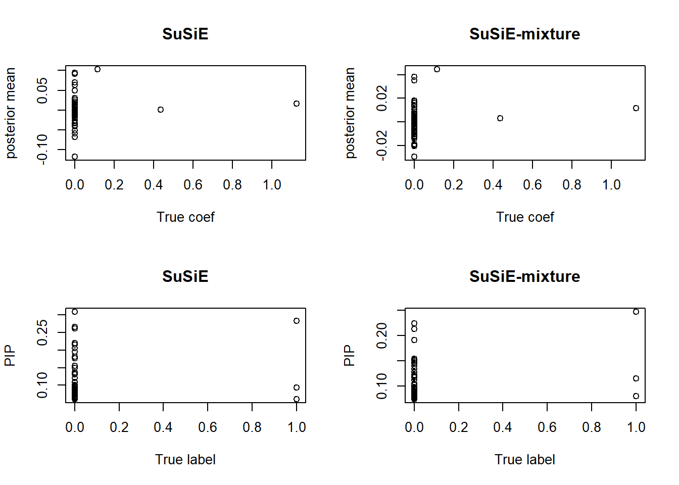
Our method gives a reasonable approximation on \(\sigma_1^2\) and \(\sigma^2\). Also, as expected, SuSiE-mixture “shrinks” the PIP of SuSiE. Theoretically, it gets less false positive, although it can be too conservative and miss discoveries.
It is also notable that, the strong shrinkage in SuSiE-mixture makes the posterior mean to be a bad estimation of the true coefficients.
sessionInfo()R version 3.6.0 (2019-04-26)
Platform: x86_64-w64-mingw32/x64 (64-bit)
Running under: Windows 10 x64 (build 17134)
Matrix products: default
locale:
[1] LC_COLLATE=English_United States.1252
[2] LC_CTYPE=English_United States.1252
[3] LC_MONETARY=English_United States.1252
[4] LC_NUMERIC=C
[5] LC_TIME=English_United States.1252
attached base packages:
[1] stats graphics grDevices utils datasets methods base
other attached packages:
[1] susieR_0.8.0
loaded via a namespace (and not attached):
[1] workflowr_1.4.0 Rcpp_1.0.1 matrixStats_0.54.0
[4] lattice_0.20-38 digest_0.6.19 rprojroot_1.3-2
[7] grid_3.6.0 backports_1.1.4 git2r_0.25.2
[10] magrittr_1.5 evaluate_0.14 stringi_1.4.3
[13] fs_1.3.1 whisker_0.3-2 Matrix_1.2-17
[16] rmarkdown_1.13 tools_3.6.0 stringr_1.4.0
[19] glue_1.3.1 xfun_0.7 yaml_2.2.0
[22] compiler_3.6.0 htmltools_0.3.6 knitr_1.23