PCA vs. t-SNE and UMAP: an illustration
Peter Carbonetto
Last updated: 2021-01-03
Checks: 7 0
Knit directory: single-cell-topics/analysis/
This reproducible R Markdown analysis was created with workflowr (version 1.6.2.9000). The Checks tab describes the reproducibility checks that were applied when the results were created. The Past versions tab lists the development history.
Great! Since the R Markdown file has been committed to the Git repository, you know the exact version of the code that produced these results.
Great job! The global environment was empty. Objects defined in the global environment can affect the analysis in your R Markdown file in unknown ways. For reproduciblity it’s best to always run the code in an empty environment.
The command set.seed(1) was run prior to running the code in the R Markdown file. Setting a seed ensures that any results that rely on randomness, e.g. subsampling or permutations, are reproducible.
Great job! Recording the operating system, R version, and package versions is critical for reproducibility.
Nice! There were no cached chunks for this analysis, so you can be confident that you successfully produced the results during this run.
Great job! Using relative paths to the files within your workflowr project makes it easier to run your code on other machines.
Great! You are using Git for version control. Tracking code development and connecting the code version to the results is critical for reproducibility.
The results in this page were generated with repository version bf01def. See the Past versions tab to see a history of the changes made to the R Markdown and HTML files.
Note that you need to be careful to ensure that all relevant files for the analysis have been committed to Git prior to generating the results (you can use wflow_publish or wflow_git_commit). workflowr only checks the R Markdown file, but you know if there are other scripts or data files that it depends on. Below is the status of the Git repository when the results were generated:
Ignored files:
    Ignored:    data/droplet.RData
    Ignored:    data/pbmc_68k.RData
    Ignored:    data/pbmc_purified.RData
    Ignored:    data/pulseseq.RData
    Ignored:    output/droplet/diff-count-droplet.RData
    Ignored:    output/droplet/fits-droplet.RData
    Ignored:    output/droplet/rds/
    Ignored:    output/pbmc-68k/fits-pbmc-68k.RData
    Ignored:    output/pbmc-68k/rds/
    Ignored:    output/pbmc-purified/diff-count-pbmc-purified.RData
    Ignored:    output/pbmc-purified/fits-pbmc-purified.RData
    Ignored:    output/pbmc-purified/rds/
    Ignored:    output/pulseseq/diff-count-pulseseq.RData
    Ignored:    output/pulseseq/fits-pulseseq.RData
    Ignored:    output/pulseseq/rds/

Untracked files:
    Untracked:  plots/

Unstaged changes:
    Modified:   TODO.txt
    Modified:   analysis/clusters_purified_pbmc.Rmd
    Modified:   analysis/diff_count_droplet.Rmd
    Modified:   analysis/diff_count_pulseseq.Rmd
    Modified:   analysis/plots_pbmc.Rmd
    Modified:   analysis/plots_tracheal_epithelium.Rmd
Note that any generated files, e.g. HTML, png, CSS, etc., are not included in this status report because it is ok for generated content to have uncommitted changes.
These are the previous versions of the repository in which changes were made to the R Markdown (analysis/pca_vs_tsne.Rmd) and HTML (docs/pca_vs_tsne.html) files. If you’ve configured a remote Git repository (see ?wflow_git_remote), click on the hyperlinks in the table below to view the files as they were in that past version.
| File | Version | Author | Date | Message |
|---|---|---|---|---|
| Rmd | bf01def | Peter Carbonetto | 2021-01-03 | workflowr::wflow_publish(“pca_vs_tsne.Rmd”) |
| Rmd | 83151f0 | Peter Carbonetto | 2021-01-03 | workflowr::wflow_publish(“index.Rmd”) |
Here we contrast use of a simple linear dimensionality reduction technique, PCA, with nonlinear dimensionality reduction methods t-SNE and UMAP.
Load the packages used in the analysis below.
library(Matrix)
library(fastTopics)
library(Rtsne)
library(uwot)
library(ggplot2)
library(cowplot)
Load the count data, the \(K = 6\) topic model fit, and the 8 clusters identified in the clustering analysis
load("../data/pbmc_purified.RData")
fit <- readRDS(file.path("../output/pbmc-purified/rds",
                         "fit-pbmc-purified-scd-ex-k=6.rds"))$fit
fit <- poisson2multinom(fit)
samples <- readRDS("../output/pbmc-purified/clustering-pbmc-purified.rds")
To begin, draw a random subset of 2,000 cells from the B, CD14+ and CD34+ clusters identified above. (The main reason for taking a random subset is that we don’t want to wait a long time for t-SNE and UMAP to complete.)
set.seed(5)
rows <- which(with(samples,
                   cluster == "B" |
                   cluster == "CD14+" |
                   cluster == "CD34+"))
rows <- sort(sample(rows,2000))
fit2 <- select_loadings(fit,loadings = rows)
x    <- samples$cluster[rows,drop = TRUE]
Next, run PCA on the topic proportions for this random subset of 2,000 samples.
p1 <- pca_plot(fit2,fill = x) + labs(fill = "cluster")Run t-SNE on the topic proportions.
tsne <- Rtsne(fit2$L,dims = 2,pca = FALSE,normalize = FALSE,perplexity = 100,
              theta = 0.1,max_iter = 1000,eta = 200,verbose = FALSE)
tsne$x <- tsne$Y
colnames(tsne$x) <- c("tsne1","tsne2")
p2 <- pca_plot(fit2,out.pca = tsne,fill = x) + labs(fill = "cluster")
Then run UMAP on the topic proportions.
out.umap <- umap(fit2$L,n_neighbors = 30,metric = "euclidean",n_epochs = 1000,
                 min_dist = 0.1,scale = "none",learning_rate = 1,
                 verbose = FALSE)
out.umap <- list(x = out.umap)
colnames(out.umap$x) <- c("umap1","umap2")
p3 <- pca_plot(fit2,out.pca = out.umap,fill = x) + labs(fill = "cluster")
Here are the PCA, t-SNE and UMAP 2-d embeddings, side-by-side:
plot_grid(p1,p2,p3,nrow = 1)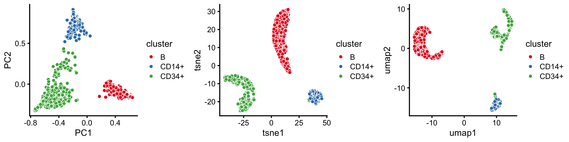
By the projection of the samples onto the first two PCs, the B-cells cluster is distinct from the others, whereas the CD14+ and CD34+ cells do not separate as well.
By contrast, this detail is not captured in the t-SNE and UMAP embeddings. This illustrates the tendency of t-SNE and UMAP to accentuate clusters in the data at the risk of distorting or obscuring finer scale substructure.
Note that the first 2 PCs should be sufficient for capturing the full structure in the topic proportions as they explain >96% of the variance:
summary(prcomp(fit2$L))
# Importance of components:
#                           PC1    PC2     PC3     PC4     PC5      PC6
# Standard deviation     0.4831 0.3269 0.10351 0.03397 0.02396 3.49e-16
# Proportion of Variance 0.6618 0.3030 0.03038 0.00327 0.00163 0.00e+00
# Cumulative Proportion  0.6618 0.9647 0.99510 0.99837 1.00000 1.00e+00
sessionInfo()
# R version 3.6.2 (2019-12-12)
# Platform: x86_64-apple-darwin15.6.0 (64-bit)
# Running under: macOS Catalina 10.15.7
#
# Matrix products: default
# BLAS:   /Library/Frameworks/R.framework/Versions/3.6/Resources/lib/libRblas.0.dylib
# LAPACK: /Library/Frameworks/R.framework/Versions/3.6/Resources/lib/libRlapack.dylib
#
# locale:
# [1] en_US.UTF-8/en_US.UTF-8/en_US.UTF-8/C/en_US.UTF-8/en_US.UTF-8
#
# attached base packages:
# [1] stats     graphics  grDevices utils     datasets  methods   base
#
# other attached packages:
# [1] cowplot_1.0.0     ggplot2_3.3.0     uwot_0.1.8        Rtsne_0.15
# [5] fastTopics_0.4-11 Matrix_1.2-18
#
# loaded via a namespace (and not attached):
#  [1] ggrepel_0.9.0        Rcpp_1.0.5           lattice_0.20-38
#  [4] FNN_1.1.3            tidyr_1.0.0          prettyunits_1.1.1
#  [7] assertthat_0.2.1     zeallot_0.1.0        rprojroot_1.3-2
# [10] digest_0.6.23        R6_2.4.1             backports_1.1.5
# [13] MatrixModels_0.4-1   evaluate_0.14        coda_0.19-3
# [16] httr_1.4.2           pillar_1.4.3         rlang_0.4.5
# [19] progress_1.2.2       lazyeval_0.2.2       data.table_1.12.8
# [22] irlba_2.3.3          SparseM_1.78         whisker_0.4
# [25] rmarkdown_2.3        labeling_0.3         stringr_1.4.0
# [28] htmlwidgets_1.5.1    munsell_0.5.0        compiler_3.6.2
# [31] httpuv_1.5.2         xfun_0.11            pkgconfig_2.0.3
# [34] mcmc_0.9-6           htmltools_0.4.0      tidyselect_0.2.5
# [37] tibble_2.1.3         workflowr_1.6.2.9000 quadprog_1.5-8
# [40] viridisLite_0.3.0    crayon_1.3.4         dplyr_0.8.3
# [43] withr_2.1.2          later_1.0.0          MASS_7.3-51.4
# [46] grid_3.6.2           jsonlite_1.6         gtable_0.3.0
# [49] lifecycle_0.1.0      git2r_0.26.1         magrittr_1.5
# [52] scales_1.1.0         RcppParallel_4.4.2   stringi_1.4.3
# [55] farver_2.0.1         fs_1.3.1             promises_1.1.0
# [58] vctrs_0.2.1          tools_3.6.2          glue_1.3.1
# [61] purrr_0.3.3          hms_0.5.2            yaml_2.2.0
# [64] colorspace_1.4-1     plotly_4.9.2         knitr_1.26
# [67] quantreg_5.54        MCMCpack_1.4-5