NMF analysis of the LPS data set

Last updated: 2025-08-20

Checks: 6 1

Knit directory: single-cell-jamboree/analysis/

This reproducible R Markdown analysis was created with workflowr (version 1.7.1). The Checks tab describes the reproducibility checks that were applied when the results were created. The Past versions tab lists the development history.

R Markdown file: up-to-date

Great! Since the R Markdown file has been committed to the Git repository, you know the exact version of the code that produced these results.

Environment: empty

Great job! The global environment was empty. Objects defined in the global environment can affect the analysis in your R Markdown file in unknown ways. For reproduciblity it’s best to always run the code in an empty environment.

Seed: set.seed(1)

The command set.seed(1) was run prior to running the code in the R Markdown file. Setting a seed ensures that any results that rely on randomness, e.g. subsampling or permutations, are reproducible.

Session information: recorded

Great job! Recording the operating system, R version, and package versions is critical for reproducibility.

Cache: detected

The following chunks had caches available:

fit-topic-model
fit-topic-model-k9
flashier-nmf-cc
flashier-nmf-k15
flashier-nmf-k9

To ensure reproducibility of the results, delete the cache directory lps_cache and re-run the analysis. To have workflowr automatically delete the cache directory prior to building the file, set delete_cache = TRUE when running wflow_build() or wflow_publish().

File paths: relative

Great job! Using relative paths to the files within your workflowr project makes it easier to run your code on other machines.

Repository version: f1c915b

Great! You are using Git for version control. Tracking code development and connecting the code version to the results is critical for reproducibility.

The results in this page were generated with repository version f1c915b. See the Past versions tab to see a history of the changes made to the R Markdown and HTML files.

Note that you need to be careful to ensure that all relevant files for the analysis have been committed to Git prior to generating the results (you can use wflow_publish or wflow_git_commit). workflowr only checks the R Markdown file, but you know if there are other scripts or data files that it depends on. Below is the status of the Git repository when the results were generated:


Untracked files:
    Untracked:  analysis/lps_cache/
    Untracked:  analysis/lps_fl_nmf_cc_k10.csv
    Untracked:  analysis/lps_gsea_fl_nmf_cc_k10.csv
    Untracked:  analysis/mcf7_cache/
    Untracked:  analysis/pancreas_cytokine_S1_factors_cache/
    Untracked:  analysis/pancreas_cytokine_lsa_clustering_cache/
    Untracked:  data/GSE125162_ALL-fastqTomat0-Counts.tsv.gz
    Untracked:  data/GSE132188_adata.h5ad.h5
    Untracked:  data/GSE156175_RAW/
    Untracked:  data/GSE183010/
    Untracked:  data/Immune_ALL_human.h5ad
    Untracked:  data/pancreas_cytokine.RData
    Untracked:  data/pancreas_cytokine_lsa.RData
    Untracked:  data/pancreas_cytokine_lsa_v2.RData
    Untracked:  data/pancreas_endocrine.RData
    Untracked:  data/pancreas_endocrine_alldays.h5ad
    Untracked:  data/yeast.RData
    Untracked:  output/panc_cyto_lsa_res/

Note that any generated files, e.g. HTML, png, CSS, etc., are not included in this status report because it is ok for generated content to have uncommitted changes.

These are the previous versions of the repository in which changes were made to the R Markdown (analysis/lps.Rmd) and HTML (docs/lps.html) files. If you’ve configured a remote Git repository (see ?wflow_git_remote), click on the hyperlinks in the table below to view the files as they were in that past version.

File	Version	Author	Date	Message
Rmd	f1c915b	Peter Carbonetto	2025-08-20	wflow_publish("lps.Rmd", verbose = T, view = F)
html	ba89f18	Peter Carbonetto	2025-08-16	Ran wflow_publish("lps.Rmd").
Rmd	a13c906	Peter Carbonetto	2025-08-16	wflow_publish("lps.Rmd", view = F, verbose = T)
Rmd	62e1130	Peter Carbonetto	2025-08-16	Updated the GSEA to use factor 10 from the fl_nmf_cc model fit in lps.Rmd.
Rmd	923976b	Peter Carbonetto	2025-08-15	In lps.Rmd, added additional MF analysis using selected pn factors; also updated the umap plots.
html	63aa311	Peter Carbonetto	2025-08-13	Ran wflow_publish("lps.Rmd").
Rmd	daa0c2d	Peter Carbonetto	2025-08-13	wflow_publish("lps.Rmd", verbose = T, view = F)
Rmd	71595a0	Peter Carbonetto	2025-08-13	Working on code for adding ‘cross-cutting’ factors to flashier model in lps analysis.
Rmd	46c7c87	Peter Carbonetto	2025-08-13	Revised a couple of the Structure plots in the lps analysis.
Rmd	83ce75d	Peter Carbonetto	2025-08-12	Started initial steps for processing of budding yeast data (GSE125162).
Rmd	4efb167	Peter Carbonetto	2025-08-04	Working on incorporating the new flashier_nmf implementation into the lps analysis.
Rmd	4887c84	Peter Carbonetto	2025-07-23	Added new gsea result from lps analysis (lps_gsea_fl_nmf_k6.csv).
Rmd	17e427e	Peter Carbonetto	2025-07-23	Added some code to save another output from the lps analysis.
html	de50dc2	Peter Carbonetto	2025-07-17	Added some histograms showing the enrichment of the IFN-a/b genes in
Rmd	d11223e	Peter Carbonetto	2025-07-17	wflow_publish("lps.Rmd", view = F, verbose = T)
html	34e8a3a	Peter Carbonetto	2025-07-16	Switched to using the flashier_nmf function from the
Rmd	9682c18	Peter Carbonetto	2025-07-16	wflow_publish("lps.Rmd", view = F, verbose = T)
html	61bec23	Peter Carbonetto	2025-07-11	Added some UMAP plots to the lps analysis.
Rmd	d35b952	Peter Carbonetto	2025-07-11	wflow_publish("lps.Rmd", view = F, verbose = T)
Rmd	9147de4	Peter Carbonetto	2025-07-04	Fixed a bug in lps.Rmd.
Rmd	3d8a2aa	Peter Carbonetto	2025-07-04	Added lps_gsea_fl_nmf.csv output.
html	e558f17	Peter Carbonetto	2025-07-04	Ran wflow_publish("lps.Rmd").
Rmd	3d27ef8	Peter Carbonetto	2025-07-04	Added GSEA of factor k6 to the lps analysis.
Rmd	cafd86d	Peter Carbonetto	2025-07-04	Implemented draft pathway analysis in temp4.R; next need to incorporate into lps.Rmd.
Rmd	b7aff59	Peter Carbonetto	2025-07-01	Added some scatterplots to compare topics and factors in the lps analysis.
Rmd	31afa30	Peter Carbonetto	2025-06-30	Added some notes/thoughts to lps.Rmd.
Rmd	23d0a0c	Peter Carbonetto	2025-06-30	Fixed one of the structure plots in the lps analysis.
Rmd	842772b	Peter Carbonetto	2025-06-30	Added k=9 fits for the topic model and flashier NMF to the lps analysis.
Rmd	eb06be5	Peter Carbonetto	2025-06-30	Added a structure plot for the k=9 topic model to the lps analysis.
Rmd	3bfc932	Peter Carbonetto	2025-06-27	Added a note to lps.Rmd.
Rmd	53085f1	Peter Carbonetto	2025-06-26	Working on adding a new topic model fit with k=9 topics in the lps example to illutrate some key ideas.
Rmd	ce314bb	Peter Carbonetto	2025-06-09	First try at running fastTopics and flashier on the pancreas_cytokine data, for mouse = S1 only; from this analysis I learned that I need to remove the mt and rp genes.
html	4abf00c	Peter Carbonetto	2025-06-06	Ran wflow_publish("lps.Rmd").
Rmd	f38b586	Peter Carbonetto	2025-06-06	A small fix to the lps analysis.
Rmd	aae4257	Peter Carbonetto	2025-06-06	A couple fixes to the lps analysis.
Rmd	6cbad5f	Peter Carbonetto	2025-06-06	Added a structure plot to the lps analysis.
Rmd	90d6c06	Peter Carbonetto	2025-06-06	Improved the structure plots in the lps analysis.
Rmd	dac95b5	Peter Carbonetto	2025-06-06	Made a few changes to the flashier fit in the lps analysis.
Rmd	9e1f127	Peter Carbonetto	2025-06-05	Added code to pancreas_cytokine analysis to prepare the scrna-seq data downloaded from geo.
Rmd	8d945a1	Peter Carbonetto	2025-06-04	Added flashier fit to lps analysis; need to revise this and the topic modeling result.
Rmd	dac6198	Peter Carbonetto	2025-06-04	Working on topic modeling results for lps data.
Rmd	8f39607	Peter Carbonetto	2025-06-04	Added steps to the lps analysis to load and prepare the data.
html	2bfef0b	Peter Carbonetto	2025-06-04	First build of the LPS analysis.
Rmd	85adf3f	Peter Carbonetto	2025-06-04	wflow_publish("lps.Rmd")

Here we will revisit the LPS data set that we analyzed using a topic model in the Takahama et al Nat Immunol paper (LPS = lipopolysaccharide). I believe some interesting insights can be gained by examining this data set more deeply.

Load packages used to process the data, perform the analyses, and create the plots.

library(Matrix)
library(readr)
library(data.table)
library(fastTopics)
library(NNLM)
library(ebnm)
library(flashier)
library(pathways)
library(singlecelljamboreeR)
library(ggplot2)
library(ggrepel)
library(cowplot)
library(rsvd)
library(uwot)

Prepare the data for analysis with fastTopics and flashier

Load the RNA-seq counts:

read_lps_data <- function (file) {
  counts <- fread(file)
  class(counts) <- "data.frame"
  genes <- counts[,1]
  counts <- t(as.matrix(counts[,-1]))
  colnames(counts) <- genes
  samples <- rownames(counts)
  samples <- strsplit(samples,"_")
  samples <- data.frame(tissue    = sapply(samples,"[[",1),
                        timepoint = sapply(samples,"[[",2),
                        mouse     = sapply(samples,"[[",3))
  samples <- transform(samples,
                       tissue    = factor(tissue),
                       timepoint = factor(timepoint),
                       mouse     = factor(mouse))
  return(list(samples = samples,counts = counts))
}
out <- read_lps_data("../data/lps.csv.gz")
samples <- out$samples
counts  <- out$counts
rm(out)

Remove a sample that appears to be an outlier based on the NMF analyses:

i       <- which(rownames(counts) != "iLN_d2_20")
samples <- samples[i,]
counts  <- counts[i,]

Remove genes that are expressed in fewer than 5 samples:

j <- which(colSums(counts > 0) > 4)
counts <- counts[,j]

This is the dimension of the data set we will analyze:

dim(counts)
# [1]   363 33533

For the Gaussian-based analyses, we will need the shifted log counts:

a <- 1
s <- rowSums(counts)
s <- s/mean(s)
shifted_log_counts <- log1p(counts/(a*s))

Topic model (fastTopics)

First let’s fit a topic model with $K = 9$ topics to the counts. This is probably an insufficient number of topics to fully capture the interesting structure in the data, but this is done on purpose since I want to illustrate how the topic model prioritizes the structure.

set.seed(1)
tm_k9 <- fit_poisson_nmf(counts,k = 9,init.method = "random",method = "em",
                         numiter = 20,verbose = "none",
                         control = list(numiter=4,nc=8,extrapolate=FALSE))
tm_k9 <- fit_poisson_nmf(counts,fit0 = tm_k9,method = "scd",numiter = 40,
                         control = list(numiter = 4,nc = 8,extrapolate = TRUE),
                         verbose = "none")

Warning: The above code chunk cached its results, but it won’t be re-run if previous chunks it depends on are updated. If you need to use caching, it is highly recommended to also set knitr::opts_chunk$set(autodep = TRUE) at the top of the file (in a chunk that is not cached). Alternatively, you can customize the option dependson for each individual chunk that is cached. Using either autodep or dependson will remove this warning. See the knitr cache options for more details.

Structure plot comparing the topics to the tissue types:

rows <- order(samples$timepoint)
topic_colors <- c("magenta","darkorange","darkblue","forestgreen",
                  "dodgerblue","gray","red","olivedrab","darkmagenta",
                  "sienna","limegreen","royalblue","lightskyblue",
                  "gold")
samples <- transform(samples,
  tissue = factor(tissue,c("PBMC","BM","CO","SI","iLN","SP",
                           "TH","SK","BR","LI","HE","KI","LU")))
structure_plot(tm_k9,grouping = samples$tissue,gap = 4,
               topics = 1:9,colors = topic_colors,
               loadings_order = rows) +
  labs(fill = "") +
  theme(axis.text.x = element_text(angle = 0,hjust = 0.5))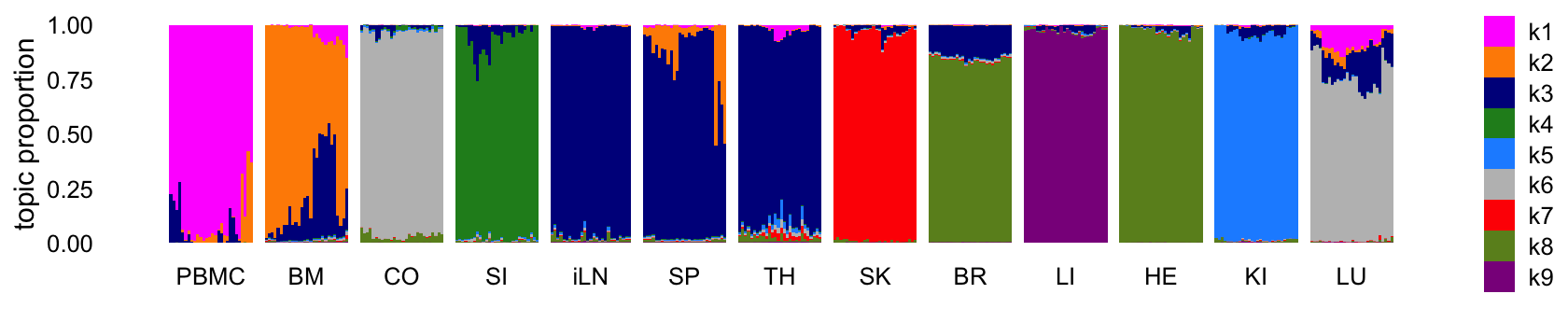

Version	Author	Date
e558f17	Peter Carbonetto	2025-07-04

Abbreviations used: BM = bone marrow; BR = brain; CO = colon; HE = heart; iLN = inguinal lymph node; KI = kidney; LI = liver; LU = lung; SI = small intestine; SK = skin; SP = spleen; TH = thymus.

The topics largely correspond to the different tissues, although because there are more tissues than topics, some tissues that are more similar to each other shared the same topic. It is also interesting that, for the most part, none of the topics are capturing changes downstream of the LPS treatment. So presumably these expression changes are more subtle than the differences in expression among the tissues.

Fit a topic model with $K = 14$ topics to the counts:

set.seed(1)
tm <- fit_poisson_nmf(counts,k = 14,init.method = "random",method = "em",
                      numiter = 20,verbose = "none",
                      control = list(numiter = 4,nc = 8,extrapolate = FALSE))
tm <- fit_poisson_nmf(counts,fit0 = tm,method = "scd",numiter = 40,
                      control = list(numiter = 4,nc = 8,extrapolate = TRUE),
                      verbose = "none")

Structure plot comparing the topics to the tissue types:

structure_plot(tm,grouping = samples$tissue,gap = 4,
               topics = 1:14,colors = topic_colors,
               loadings_order = rows) +
  labs(fill = "") +
  theme(axis.text.x = element_text(angle = 0,hjust = 0.5),
        legend.key.height = unit(0.01,"cm"),
        legend.key.width = unit(0.2,"cm"),
        legend.text = element_text(size = 6))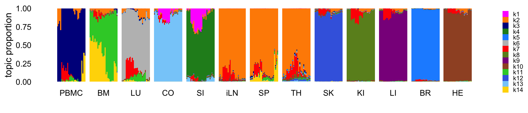

Version	Author	Date
e558f17	Peter Carbonetto	2025-07-04
4abf00c	Peter Carbonetto	2025-06-06

This next structure plot better highlights the topics that are capturing expression changes over time, some being presumably driven by the LPS-induced sepsis:

topic_colors <- c("magenta","gray50","gray65","gray40",
                  "gray85","gray75","red","gray80","gray90",
                  "gray60","limegreen","gray70","gray55",
                  "gold")
structure_plot(tm,grouping = samples$tissue,gap = 4,
               topics = 1:14,colors = topic_colors,
               loadings_order = rows) +
  labs(fill = "") +
  theme(axis.text.x = element_text(angle = 0,hjust = 0.5),
        legend.key.height = unit(0.01,"cm"),
        legend.key.width = unit(0.2,"cm"),
        legend.text = element_text(size = 6))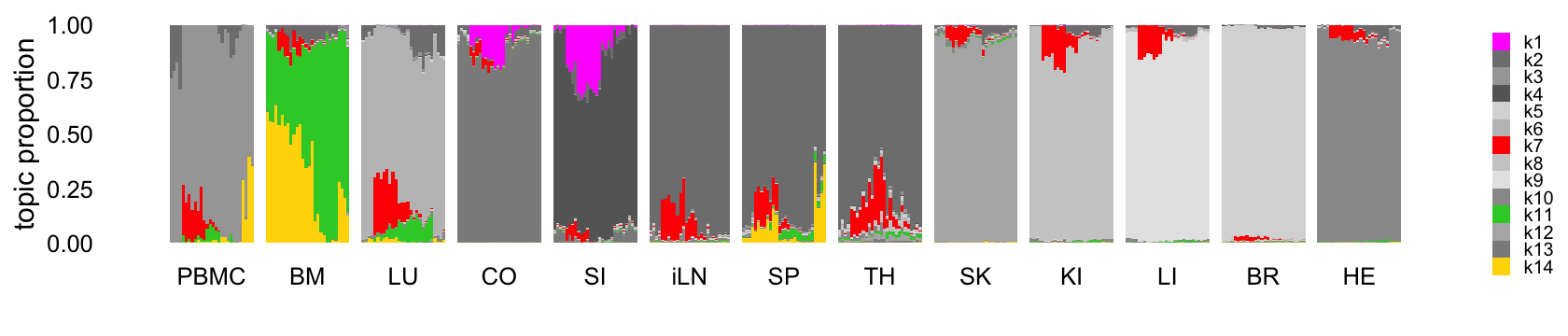

Version	Author	Date
e558f17	Peter Carbonetto	2025-07-04
4abf00c	Peter Carbonetto	2025-06-06

EBNMF (flashier)

Similar to the topic modeling analysis, let’s start by fitting an EBNMF to the shifted log counts using flashier, first with $K = 9$. Since the greedy initialization does not seem to work well in this example, I’ll use a different initialization strategy: obtain a “good” initialization using the NNLM package, then use this initialization to fit a NMF using flashier. This approach is implemented in the following function:

Now fit an NMF to the shifted log counts, with $K = 9$:

set.seed(1)
n  <- nrow(shifted_log_counts)
x  <- rpois(1e7,1/n)
s1 <- sd(log(x + 1))
set.seed(1)
fl_nmf_k9 <- flashier_nmf(shifted_log_counts,k = 9,greedy_init = TRUE,
                          var_type = 2,S = s1,verbose = 0)

Structure plot comparing the topics to the tissue types:

rows <- order(samples$timepoint)
topic_colors <- c("powderblue","darkorange","olivedrab","limegreen",
                  "forestgreen","cyan","darkmagenta","gray","dodgerblue",
                  "red","gold","darkblue","lightskyblue",
                  "royalblue","sienna")
L <- ldf(fl_nmf_k9,type = "i")$L
structure_plot(L,grouping = samples$tissue,gap = 4,
               topics = 1:9,colors = topic_colors,
               loadings_order = rows) +
  labs(fill = "",y = "membership")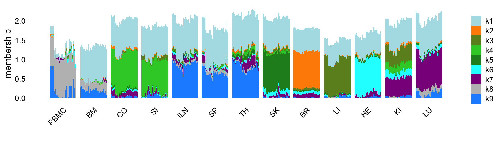

Version	Author	Date
63aa311	Peter Carbonetto	2025-08-13
e558f17	Peter Carbonetto	2025-07-04

Like the topic model, the EBNMF model with $K = 9$ does not capture any changes downstream of the LPS-induced sepsis.

Next fit an NMF to the shifted log counts using flashier, with $K = 15$:

set.seed(1)
fl_nmf <- flashier_nmf(shifted_log_counts,k = 15,greedy_init = TRUE,
                       var_type = 2,S = s1,verbose = 0)

Structure plot comparing the factors to the tissue types:

L <- ldf(fl_nmf,type = "i")$L
structure_plot(L,grouping = samples$tissue,gap = 4,
               topics = 1:15,colors = topic_colors,
               loadings_order = rows) +
  labs(fill = "",y = "membership") +
  theme(axis.text.x = element_text(angle = 0,hjust = 0.5),
        legend.key.height = unit(0.01,"cm"),
        legend.key.width = unit(0.25,"cm"),
        legend.text = element_text(size = 7))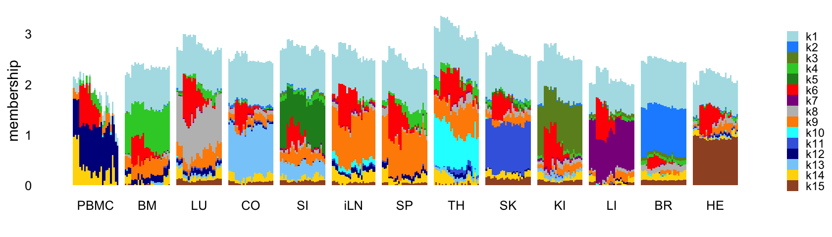

Version	Author	Date
63aa311	Peter Carbonetto	2025-08-13
34e8a3a	Peter Carbonetto	2025-07-16
e558f17	Peter Carbonetto	2025-07-04
4abf00c	Peter Carbonetto	2025-06-06

This next structure plot better highlights the topics that capture the processes that are driven or may be driven by LPS-induced sepsis:

rows <- order(samples$timepoint)
topic_colors <- c("gray95","gray70","gray80","gray50",
                  "gray60","gray90","gray75","gray","gray85",
                  "red","gold","gray65","gray45",
                  "gray35","gray75")
L <- ldf(fl_nmf,type = "i")$L
structure_plot(L,grouping = samples$tissue,gap = 4,
               topics = 1:15,colors = topic_colors,
               loadings_order = rows) +
  labs(fill = "",y = "membership") +
  theme(axis.text.x = element_text(angle = 0,hjust = 0.5),
        legend.key.height = unit(0.01,"cm"),
        legend.key.width = unit(0.25,"cm"),
        legend.text = element_text(size = 7))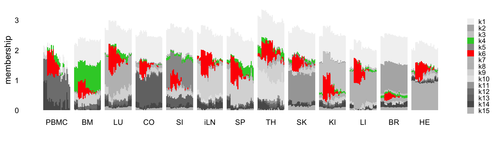

Version	Author	Date
63aa311	Peter Carbonetto	2025-08-13
34e8a3a	Peter Carbonetto	2025-07-16
e558f17	Peter Carbonetto	2025-07-04
4abf00c	Peter Carbonetto	2025-06-06

EBNMF with “cross-cutting” factor(s)

One question I have is whether it is sufficient to model increases in expression for these “cross-cutting” factors, or whether it is better to allow for both decreases in expression (negative on log-scale) and increases (positive on log-scale). Let’s test this.

cc_factors <- 10:11
nn_factors <- c(1:9,12:15)
fl_nmf_cc <- convert_factors_nn_to_pn(fl_nmf,cc_factors,shifted_log_counts,
                                      S = s1,var_type = 2)
fl_nmf_cc <- flash_backfit(fl_nmf_cc,extrapolate = FALSE,maxiter = 100,
                           verbose = 2)
fl_nmf_cc <- flash_backfit(fl_nmf_cc,extrapolate = TRUE,maxiter = 100,
                           verbose = 2)
# Backfitting 15 factors (tolerance: 1.81e-01)...
#   Difference between iterations is within 1.0e+03...
#   Difference between iterations is within 1.0e+02...
#   --Maximum number of iterations reached!
# Wrapping up...
# Done.
# Backfitting 15 factors (tolerance: 1.81e-01)...
#   Difference between iterations is within 1.0e+01...
#   --Maximum number of iterations reached!
#   Backfit complete. Objective: -3286910.603 
# Wrapping up...
# Done.

For the two cross-cutting factors, modeling both decreases and increases does seem to produce a number of decreases in expression, but overall the LFCs remain very similar:

pdat <- data.frame(nmf    = as.vector(ldf(fl_nmf,type="i")$F[,cc_factors]),
                   nmf_cc = as.vector(ldf(fl_nmf_cc,type="i")$F[,cc_factors]))
ggplot(pdat,aes(x = nmf,y = nmf_cc)) +
  geom_point() +
  geom_abline(intercept = 0,slope = 1,color = "magenta",linetype = "dotted") +
  theme_cowplot(font_size = 10)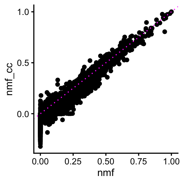

Version	Author	Date
ba89f18	Peter Carbonetto	2025-08-16

This suggests that while modeling both positive and negative changes is useful, it is perhaps not essential.

The following three plots compare: (i) F for the non-negative factors only; (ii) L for the non-negative factors only; (iii) L for the (positive and negative) cross-cutting factors. Overall, these parameter estimates did not change much.

pdat1 <- data.frame(nmf    = as.vector(ldf(fl_nmf,type="i")$F[,nn_factors]),
                    nmf_cc = as.vector(ldf(fl_nmf_cc,type="i")$F[,nn_factors]))
pdat1 <- subset(pdat1,abs(nmf) > 0.01 & abs(nmf_cc) > 0.01)
p1 <- ggplot(pdat1,aes(x = nmf,y = nmf_cc)) +
  geom_point() +
  geom_abline(intercept = 0,slope = 1,color = "magenta",linetype = "dotted") +
  theme_cowplot(font_size = 10)
pdat2 <- data.frame(nmf    = as.vector(ldf(fl_nmf,type="i")$L[,nn_factors]),
                    nmf_cc = as.vector(ldf(fl_nmf_cc,type="i")$L[,nn_factors]))
pdat2 <- subset(pdat2,abs(nmf) > 0.01 & abs(nmf_cc) > 0.01)
p2 <- ggplot(pdat2,aes(x = nmf,y = nmf_cc)) +
  geom_point() +
  geom_abline(intercept = 0,slope = 1,color = "magenta",linetype = "dotted") +
  theme_cowplot(font_size = 10)
pdat3 <- data.frame(nmf    = as.vector(ldf(fl_nmf,type="i")$L[,cc_factors]),
                    nmf_cc = as.vector(ldf(fl_nmf_cc,type="i")$L[,cc_factors]))
p3 <- ggplot(pdat3,aes(x = nmf,y = nmf_cc)) +
  geom_point() +
  geom_abline(intercept = 0,slope = 1,color = "magenta",linetype = "dotted") +
  theme_cowplot(font_size = 10)
plot_grid(p1,p2,p3,nrow = 1,ncol = 3)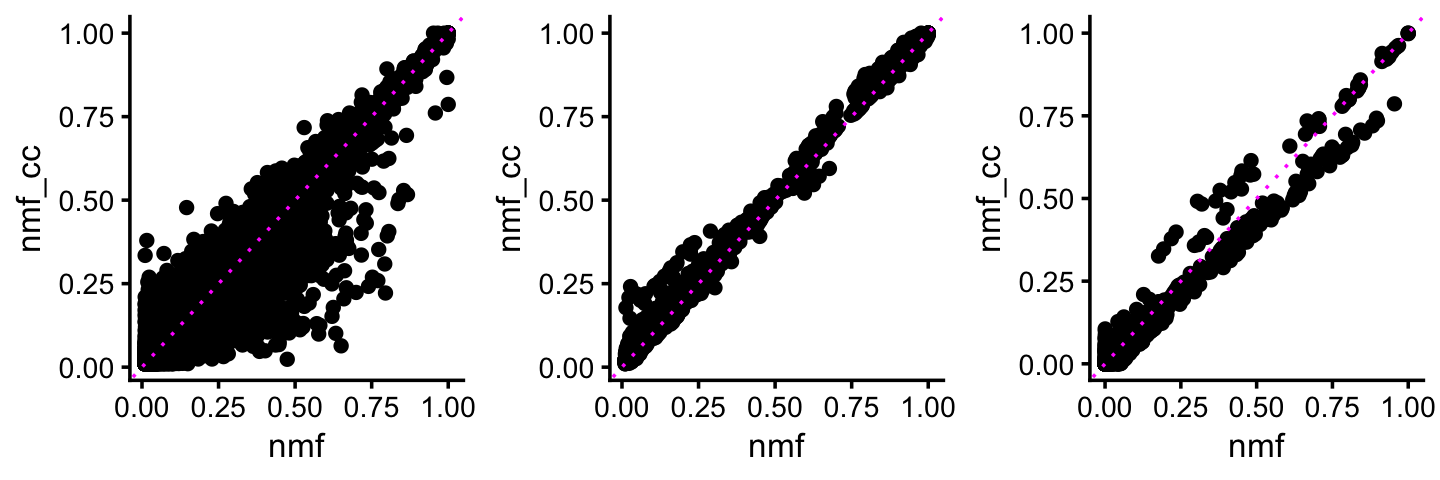

Version	Author	Date
ba89f18	Peter Carbonetto	2025-08-16

Here is the updated Structure plot, highlighting again the sepsis-related (“cross-cutting”) factors:

rows <- order(samples$timepoint)
L <- ldf(fl_nmf_cc,type = "i")$L
structure_plot(L,grouping = samples$tissue,gap = 4,
                    topics = 1:15,colors = topic_colors,
                    loadings_order = rows) +
  labs(fill = "",y = "membership") +
  theme(axis.text.x = element_text(angle = 0,hjust = 0.5),
        legend.key.height = unit(0.01,"cm"),
        legend.key.width = unit(0.25,"cm"),
        legend.text = element_text(size = 7))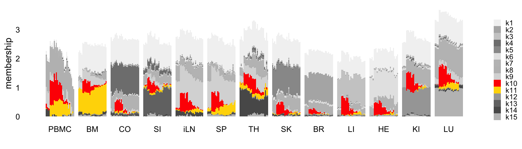

Version	Author	Date
ba89f18	Peter Carbonetto	2025-08-16

Comparison with UMAP

Here I project the samples onto a 2-d embedding using UMAP to show that this LPS-related substructure is not obvious from a UMAP plot.

set.seed(1)
U <- rsvd(shifted_log_counts,k = 40)$u
Y <- umap(U,n_neighbors = 20,metric = "cosine",min_dist = 0.3,
          n_threads = 8,verbose = FALSE)
x <- Y[,1]
y <- Y[,2]
samples$umap1 <- x
samples$umap2 <- y

I color the samples in the UMAP plot by tissue (top-left) and by membership to factor 10 (top-right, bottom-left):

tissue_colors <- c("magenta","darkorange","darkblue","forestgreen",
                   "dodgerblue","red","olivedrab","darkmagenta",
                   "sienna","limegreen","royalblue","lightskyblue",
                   "gold")
L            <- ldf(fl_nmf,type = "i")$L
colnames(L)  <- paste0("k",1:15)
pdat         <- samples
pdat$factor10 <- L[,"k10"]
pdat$topic7  <- poisson2multinom(tm)$L[,"k7"]
p1 <- ggplot(pdat,aes(x = umap1,y = umap2,color = tissue)) +
  geom_point(size = 1) +
  scale_color_manual(values = tissue_colors) +
  theme_cowplot(font_size = 10)
p2 <- ggplot(pdat,aes(x = umap1,y = umap2,color = factor10)) +
  geom_point(size = 1) +
  scale_color_gradient2(low = "deepskyblue",mid = "gold",high = "tomato",
                        midpoint = 0.66) +
  theme_cowplot(font_size = 10)
p3 <- ggplot(pdat,aes(x = umap1,y = umap2,color = topic7)) +
  geom_point(size = 1) +
  scale_color_gradient2(low = "deepskyblue",mid = "gold",high = "tomato",
                        midpoint = 0.15) +
  theme_cowplot(font_size = 10)
plot_grid(p1,p2,p3,nrow = 2,ncol = 2)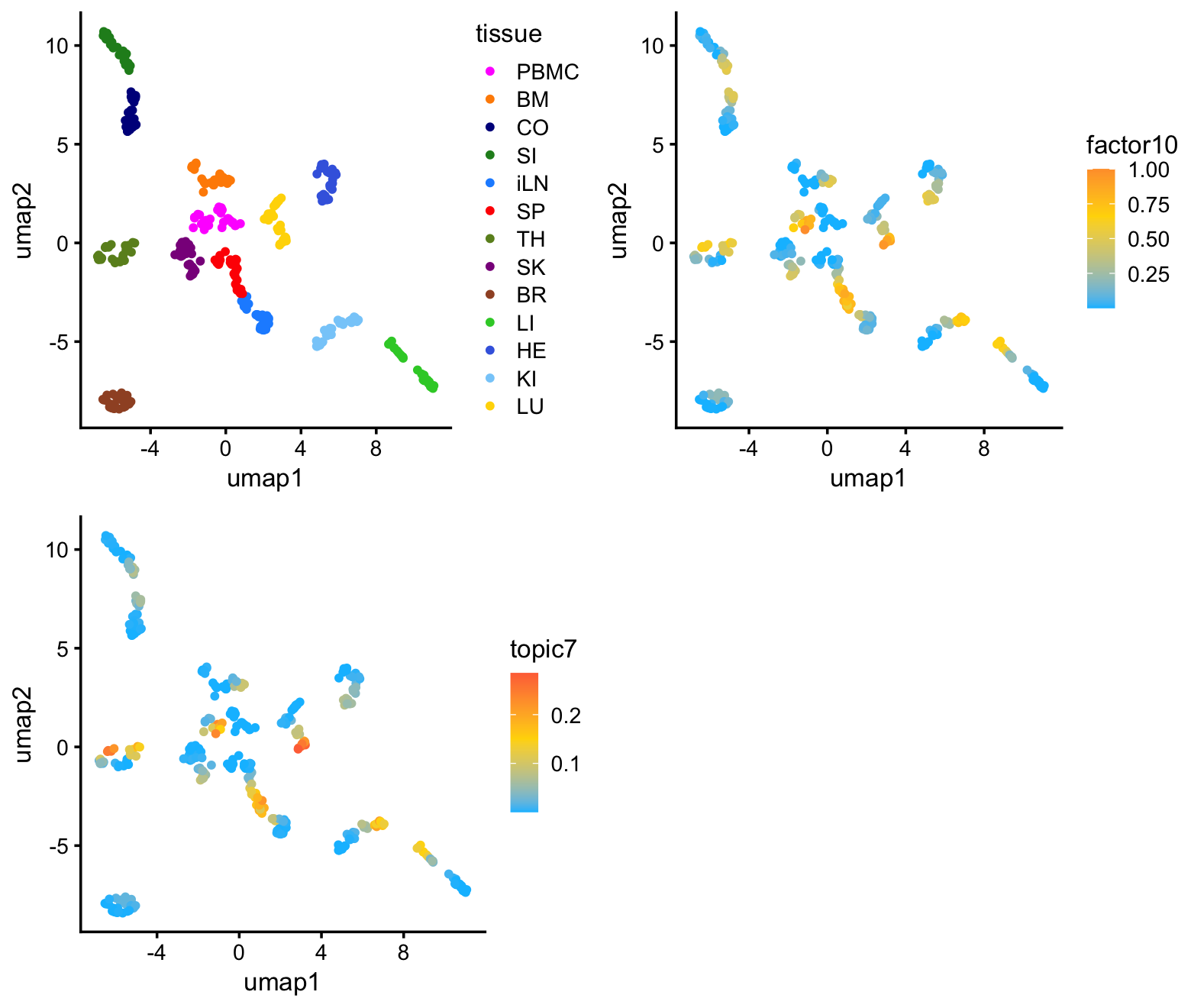

Version	Author	Date
ba89f18	Peter Carbonetto	2025-08-16
63aa311	Peter Carbonetto	2025-08-13
34e8a3a	Peter Carbonetto	2025-07-16
61bec23	Peter Carbonetto	2025-07-11

As expected, the predominant structure is due to the different tissues, with more similar tissues clustering together. There is also some more subtle structure within each cluster that appears to correspond well with factor 10 (and, correspondingly, topic 7). So althought the UMAP does seem to reveal the sepsis-related structure, it cannot isolate the sepsis-related gene expression signature.

Factors isolating responses to LPS-induced sepsis

From the Structure plots, it appears that topic 7, and possibly topic 1, are capturing processes activated by LPS. However, I conjecture that it is difficult to determine which genes should members of topic 1 and which are members of the colon and small intensine topics. Indeed, topic 1 shares many genes with these two topics:

pdat <- cbind(data.frame(gene = colnames(counts)),
              poisson2multinom(tm)$F)
rows <- which(pdat$k1 < 0.01)
pdat[rows,"gene"] <- ""
p1 <- ggplot(pdat,aes(x = k1,y = k4,label = gene)) +
  geom_point() +
  geom_text_repel(color = "gray",size = 2.5,max.overlaps = Inf) +
  scale_x_continuous(trans = "sqrt") +
  scale_y_continuous(trans = "sqrt") +
  theme_cowplot(font_size = 10)
p2 <- ggplot(pdat,aes(x = k1,y = k13,label = gene)) +
  geom_point() +
  geom_text_repel(color = "gray",size = 2.5,max.overlaps = Inf) +
  scale_x_continuous(trans = "sqrt") +
  scale_y_continuous(trans = "sqrt") +
  theme_cowplot(font_size = 10)
plot_grid(p1,p2,nrow = 1,ncol = 2)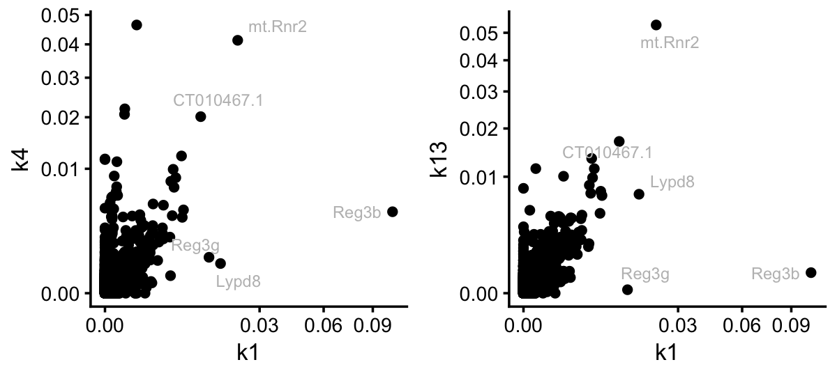

Version	Author	Date
ba89f18	Peter Carbonetto	2025-08-16
63aa311	Peter Carbonetto	2025-08-13
34e8a3a	Peter Carbonetto	2025-07-16
61bec23	Peter Carbonetto	2025-07-11
e558f17	Peter Carbonetto	2025-07-04

Still, it is interesting that three genes, Reg3b, Reg3g and Lypd8, stand out in topic 1 as distinct from the colon and SI topics. Let’s now contrast this to the situation for topic 7:

pdat <- cbind(data.frame(gene = colnames(counts)),
              poisson2multinom(tm)$F)
rows <- which(pdat$k7 < 0.008)
pdat[rows,"gene"] <- ""
p1 <- ggplot(pdat,aes(x = k7,y = k6,label = gene)) +
  geom_point() +
  geom_text_repel(color = "gray",size = 2.5,max.overlaps = Inf) +
  scale_x_continuous(trans = "sqrt") +
  scale_y_continuous(trans = "sqrt") +
  theme_cowplot(font_size = 10)
p2 <- ggplot(pdat,aes(x = k7,y = k8,label = gene)) +
  geom_point() +
  geom_text_repel(color = "gray",size = 2.5,max.overlaps = Inf) +
  scale_x_continuous(trans = "sqrt") +
  scale_y_continuous(trans = "sqrt") +
  theme_cowplot(font_size = 10)
plot_grid(p1,p2,nrow = 1,ncol = 2)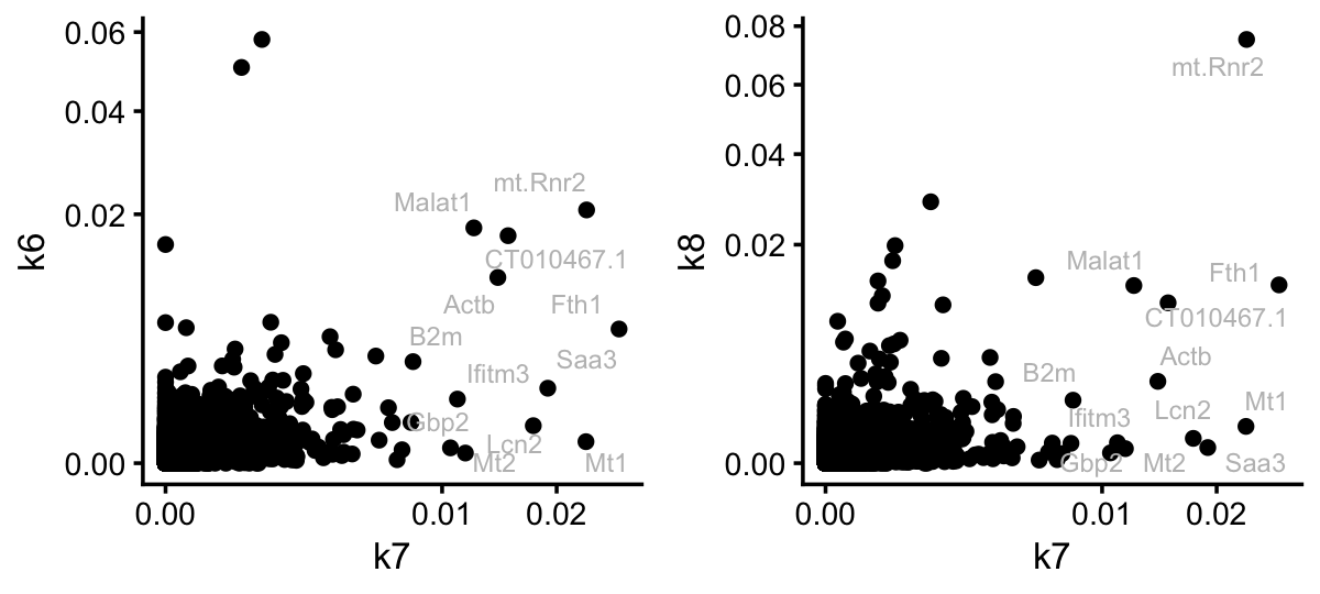

Version	Author	Date
ba89f18	Peter Carbonetto	2025-08-16
63aa311	Peter Carbonetto	2025-08-13
de50dc2	Peter Carbonetto	2025-07-17
34e8a3a	Peter Carbonetto	2025-07-16
61bec23	Peter Carbonetto	2025-07-11
e558f17	Peter Carbonetto	2025-07-04

For illustration, I compared topic 7 to the kidney and lung topics. The key point here is that the topic model has selected genes for topic 7 that are very independent of the tissue topics. So this looks quite promising. Let’s now see if the result is similar for the EBNMF model fitted to the shifted log counts:

F <- ldf(fl_nmf_cc,type = "i")$F
colnames(F) <- paste0("k",1:15)
pdat <- data.frame(tm     = poisson2multinom(tm)$F[,"k7"],
                   nmf_cc = F[,"k10"],
                   gene   = rownames(F))
rows <- which(with(pdat,tm < 0.005 & nmf_cc < 0.8))
pdat[rows,"gene"] <- ""
ggplot(pdat,aes(x = (tm)^(1/3),y = nmf_cc,label = gene)) +
  geom_point() +
  geom_text_repel(color = "gray",size = 2.5,max.overlaps = Inf) +
  labs(x = "topic 7",y = "factor 10") +
  theme_cowplot(font_size = 12)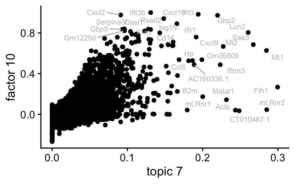

Version	Author	Date
ba89f18	Peter Carbonetto	2025-08-16

Indeed, factor 10 and topic 7 are cpaturing very similar expression patterns.

Next I ran GSEA on the on factor 10. (Running GSEA on topic 7 is complicated by the fact that it would be better to “shrink” the estimates before running GSEA, whereas this was automatically done for EBNMF result.)

data(gene_sets_mouse)
gene_sets     <- gene_sets_mouse$gene_sets
gene_info     <- gene_sets_mouse$gene_info
gene_set_info <- gene_sets_mouse$gene_set_info
j <- which(with(gene_sets_mouse$gene_set_info,
                (database == "MSigDB-C2" &
                 grepl("CP",sub_category_code,fixed = TRUE)) |
                (database == "MSigDB-C5") &
                 grepl("GO",sub_category_code,fixed = TRUE)))
genes <- sort(intersect(rownames(F),gene_info$Symbol))
i     <- which(is.element(gene_info$Symbol,genes))
gene_info     <- gene_info[i,]
gene_set_info <- gene_set_info[j,]
gene_sets     <- gene_sets[i,j]
rownames(gene_sets) <- gene_info$Symbol
rownames(gene_set_info) <- gene_set_info$id
gene_set_info <- gene_set_info[,-2]
F <- ldf(fl_nmf_cc,type = "i")$F
colnames(F) <- paste0("k",1:15)
gsea_fl_nmf_cc <- singlecelljamboreeR::perform_gsea(F[,"k10"],gene_sets,
                                                    gene_set_info,L = 15,
                                                    verbose = FALSE)
write.csv(data.frame(gene = rownames(F),signal = round(F[,"k10"],digits = 6)),
          "lps_fl_nmf_cc_k10.csv",row.names = FALSE,quote = FALSE)
out <- gsea_fl_nmf_cc$selected_gene_sets
out$top_genes <- sapply(out$top_genes,function (x) paste(x,collapse = " "))
out$lbf  <- round(out$lbf,digits = 6)
out$pip  <- round(out$pip,digits = 6)
out$coef <- round(out$coef,digits = 6)
write_csv(out,"lps_gsea_fl_nmf_cc_k10.csv",quote = "none")

The top gene set is the IFN-$\alpha/\beta$ signaling pathway, but other gene sets clearly relate to inflammation and immune system function:

print(gsea_fl_nmf_cc$selected_gene_sets[c(2:7,9)],n = Inf)
# # A tibble: 25 × 7
#    CS    gene_set   lbf    pip    coef genes name                               
#    <fct> <chr>    <dbl>  <dbl>   <dbl> <dbl> <chr>                              
#  1 L1    M973     327.  1       0.272     49 REACTOME_INTERFERON_ALPHA_BETA_SIG…
#  2 L2    M27605   171.  1       0.211     44 REACTOME_INTERLEUKIN_10_SIGNALING  
#  3 L3    M14405   113.  0.999   0.0777   222 GO_DEFENSE_RESPONSE_TO_VIRUS       
#  4 L4    M15265    79.7 1.000   0.0757   171 GO_RESPONSE_TO_INTERFERON_GAMMA    
#  5 L7    M18914    58.5 1       0.223     15 GO_CXCR_CHEMOKINE_RECEPTOR_BINDING 
#  6 L5    M13436    53.0 1.000   0.0609   186 GO_RESPONSE_TO_INTERLEUKIN_1       
#  7 L10   M17358    31.6 1.000   0.0539   157 GO_SPECIFIC_GRANULE                
#  8 L6    M39785    29.3 1.000  -0.146     20 WP_OVERVIEW_OF_INTERFERONSMEDIATED…
#  9 L9    M26883    28.5 1.000   0.168     15 GO_PROTEIN_ADP_RIBOSYLASE_ACTIVITY 
# 10 L12   M10974    27.7 0.997   0.0674    91 GO_NEGATIVE_REGULATION_OF_VIRAL_PR…
# 11 L14   M12167    22.6 0.994   0.0432   192 GO_PATTERN_RECOGNITION_RECEPTOR_SI…
# 12 L11   M39818    22.0 1.000   0.0366   264 WP_IL18_SIGNALING_PATHWAY          
# 13 L8    M15261    21.2 0.652   0.0316   345 GO_REGULATION_OF_INFLAMMATORY_RESP…
# 14 L8    M15877    21.2 0.346   0.0486   138 GO_POSITIVE_REGULATION_OF_INFLAMMA…
# 15 L13   M39618    19.5 0.998   0.109     27 WP_PHOTODYNAMIC_THERAPYINDUCED_UNF…
# 16 L15   M255      15.6 0.343   0.0644    65 PID_HIF1_TFPATHWAY                 
# 17 L15   M39678    15.6 0.249  -0.0559    86 WP_RETINOBLASTOMA_GENE_IN_CANCER   
# 18 L15   M12630    15.6 0.0935  0.0463   122 GO_TRANSITION_METAL_ION_HOMEOSTASIS
# 19 L15   M15481    15.6 0.0790  0.0508   100 GO_CELLULAR_TRANSITION_METAL_ION_H…
# 20 L15   M4217     15.6 0.0741 -0.0368   195 REACTOME_MITOTIC_PROMETAPHASE      
# 21 L15   M11809    15.6 0.0355  0.0916    28 GO_RESPONSE_TO_INTERFERON_BETA     
# 22 L15   M39363    15.6 0.0281  0.0843    33 WP_TYPE_II_INTERFERON_SIGNALING_IF…
# 23 L15   M11125    15.6 0.0248  0.0666    54 GO_NEGATIVE_REGULATION_OF_INNATE_I…
# 24 L15   M23341    15.6 0.0223  0.139     11 GO_CELLULAR_RESPONSE_TO_INTERFERON…
# 25 L15   M17276    15.6 0.0132  0.0565    74 GO_PRERIBOSOME

This is the same scatterplot as the one just above, but with the genes in the IFN-$\alpha/\beta$ signaling pathway highlighted:

pdat$pathway <- FALSE
pathway_genes <- names(which(gene_sets[,"M973"] > 0))
pdat[pathway_genes,"pathway"] <- TRUE
pdat <- pdat[order(pdat$pathway),]
ggplot(pdat,aes(x = (tm)^(1/3),y = nmf_cc,label = gene,color = pathway)) +
  geom_point() +
  geom_text_repel(color = "gray",size = 2.5,max.overlaps = Inf) +
  scale_color_manual(values = c("darkblue","orangered")) +
  labs(x = "topic 7",y = "factor 10") +
  theme_cowplot(font_size = 12)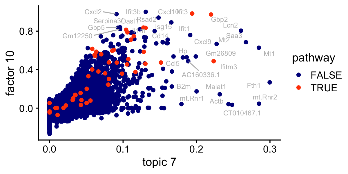

Version	Author	Date
ba89f18	Peter Carbonetto	2025-08-16

Here’s another view of the enrichment of the genes in the IFN-$\alpha/\beta$ pathway:

p1 <- ggplot(subset(pdat,pathway),aes(x = nmf_cc)) +
  geom_histogram(color = "white",fill = "black",bins = 16) +
  labs(x = "factor 10",y = "IFN-a/b genes") +
  theme_cowplot(font_size = 10)
p2 <- ggplot(subset(pdat,!pathway),aes(x = nmf_cc)) +
  geom_histogram(color = "white",fill = "black",bins = 24) +
  labs(x = "factor 10",y = "other genes") +
  theme_cowplot(font_size = 10)
p3 <- ggplot(subset(pdat,pathway),aes(x = log10(tm + 1e-6))) +
  geom_histogram(color = "white",fill = "black",bins = 16) +
  labs(x = "topic 7",y = "IFN-a/b genes") +
  theme_cowplot(font_size = 10)
p4 <- ggplot(subset(pdat,!pathway),aes(x = log10(tm + 1e-6))) +
  geom_histogram(color = "white",fill = "black",bins = 24) +
  labs(x = "topic 7",y = "other genes") +
  theme_cowplot(font_size = 10)
plot_grid(p1,p2,p3,p4,nrow = 2,ncol = 2,rel_widths = c(2,3))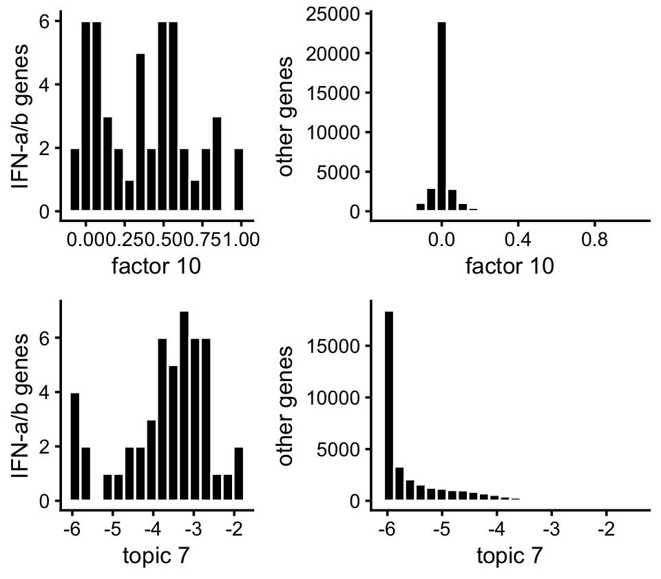

Version	Author	Date
ba89f18	Peter Carbonetto	2025-08-16

Yet another visualization of this enrichment result:

rank_random_tie <- function (x) {
  n <- length(x)
  return((rank(x,ties.method = "random",na.last = "keep") - 1)/(n-1))
}
F <- ldf(fl_nmf_cc,type = "i")$F
colnames(F) <- paste0("k",1:15)
pdat <- data.frame(factor = F[,"k10"],
                   gene   = rownames(F))
                   pdat$pathway <- FALSE
pathway_genes <- names(which(gene_sets[,"M973"] > 0))
pdat[pathway_genes,"pathway"] <- TRUE
pdat1 <- subset(pdat,pathway)
pdat2 <- subset(pdat,!pathway)
pdat1 <- transform(pdat1,rank = rank_random_tie(factor))
pdat2 <- transform(pdat2,rank = rank_random_tie(factor))
rows  <- which(pdat1$rank < 0.5)
pdat1[rows,"gene"] <- ""
pdat2[,"gene"] <- ""
pdat <- rbind(pdat1,pdat2)
ggplot(pdat,aes(x = rank,y = factor,color = pathway,label = gene)) +
  geom_point(size = 1) +
  geom_text_repel(color = "black",size = 2.5,max.overlaps = Inf,
                  min.segment.length = 0) +
  scale_y_continuous(breaks = seq(-1,1,0.2)) +
  scale_color_manual(values = c("darkblue","red")) +
  guides(color = "none") +
  labs(y = "factor 10") +
  theme_cowplot(font_size = 10)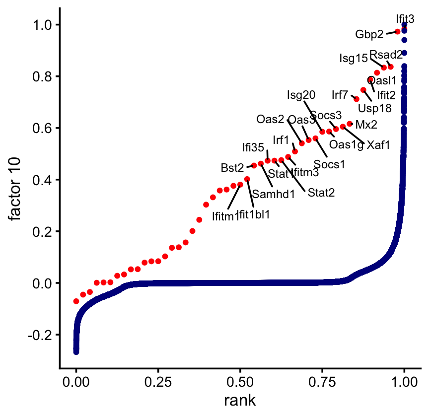

sessionInfo()
# R version 4.3.3 (2024-02-29)
# Platform: aarch64-apple-darwin20 (64-bit)
# Running under: macOS 15.5
# 
# Matrix products: default
# BLAS:   /Library/Frameworks/R.framework/Versions/4.3-arm64/Resources/lib/libRblas.0.dylib 
# LAPACK: /Library/Frameworks/R.framework/Versions/4.3-arm64/Resources/lib/libRlapack.dylib;  LAPACK version 3.11.0
# 
# locale:
# [1] en_US.UTF-8/en_US.UTF-8/en_US.UTF-8/C/en_US.UTF-8/en_US.UTF-8
# 
# time zone: America/Chicago
# tzcode source: internal
# 
# attached base packages:
# [1] stats     graphics  grDevices utils     datasets  methods   base     
# 
# other attached packages:
#  [1] uwot_0.2.3                 rsvd_1.0.5                
#  [3] cowplot_1.1.3              ggrepel_0.9.6             
#  [5] ggplot2_3.5.2              singlecelljamboreeR_0.1-39
#  [7] pathways_0.1-20            flashier_1.0.56           
#  [9] ebnm_1.1-34                NNLM_0.4.4                
# [11] fastTopics_0.7-25          data.table_1.17.6         
# [13] readr_2.1.5                Matrix_1.6-5              
# 
# loaded via a namespace (and not attached):
#   [1] pbapply_1.7-2        rlang_1.1.6          magrittr_2.0.3      
#   [4] git2r_0.33.0         RcppAnnoy_0.0.22     horseshoe_0.2.0     
#   [7] matrixStats_1.2.0    susieR_0.14.18       compiler_4.3.3      
#  [10] vctrs_0.6.5          reshape2_1.4.4       RcppZiggurat_0.1.6  
#  [13] quadprog_1.5-8       stringr_1.5.1        pkgconfig_2.0.3     
#  [16] crayon_1.5.3         fastmap_1.2.0        labeling_0.4.3      
#  [19] utf8_1.2.6           promises_1.3.3       rmarkdown_2.29      
#  [22] tzdb_0.4.0           bit_4.0.5            purrr_1.0.4         
#  [25] Rfast_2.1.0          xfun_0.52            cachem_1.1.0        
#  [28] trust_0.1-8          jsonlite_2.0.0       progress_1.2.3      
#  [31] later_1.4.2          reshape_0.8.9        BiocParallel_1.36.0 
#  [34] irlba_2.3.5.1        parallel_4.3.3       prettyunits_1.2.0   
#  [37] R6_2.6.1             bslib_0.9.0          stringi_1.8.7       
#  [40] RColorBrewer_1.1-3   SQUAREM_2021.1       jquerylib_0.1.4     
#  [43] Rcpp_1.1.0           knitr_1.50           R.utils_2.12.3      
#  [46] httpuv_1.6.14        splines_4.3.3        tidyselect_1.2.1    
#  [49] dichromat_2.0-0.1    yaml_2.3.10          codetools_0.2-19    
#  [52] lattice_0.22-5       tibble_3.3.0         plyr_1.8.9          
#  [55] withr_3.0.2          evaluate_1.0.4       Rtsne_0.17          
#  [58] RcppParallel_5.1.10  pillar_1.11.0        whisker_0.4.1       
#  [61] plotly_4.11.0        softImpute_1.4-3     generics_0.1.4      
#  [64] vroom_1.6.5          rprojroot_2.0.4      invgamma_1.2        
#  [67] truncnorm_1.0-9      hms_1.1.3            scales_1.4.0        
#  [70] ashr_2.2-66          gtools_3.9.5         RhpcBLASctl_0.23-42 
#  [73] glue_1.8.0           scatterplot3d_0.3-44 lazyeval_0.2.2      
#  [76] tools_4.3.3          fgsea_1.35.4         fs_1.6.6            
#  [79] fastmatch_1.1-6      grid_4.3.3           tidyr_1.3.1         
#  [82] colorspace_2.1-0     deconvolveR_1.2-1    cli_3.6.5           
#  [85] Polychrome_1.5.1     workflowr_1.7.1      mixsqp_0.3-54       
#  [88] viridisLite_0.4.2    dplyr_1.1.4          gtable_0.3.6        
#  [91] R.methodsS3_1.8.2    sass_0.4.10          digest_0.6.37       
#  [94] htmlwidgets_1.6.4    farver_2.1.2         R.oo_1.26.0         
#  [97] htmltools_0.5.8.1    lifecycle_1.0.4      httr_1.4.7          
# [100] bit64_4.0.5

NMF analysis of the LPS data set

Peter Carbonetto

Prepare the data for analysis with fastTopics and flashier

Topic model (fastTopics)

EBNMF (flashier)

EBNMF with “cross-cutting” factor(s)

Comparison with UMAP

Factors isolating responses to LPS-induced sepsis