Initial exploration of the human brain dataset: committed OPC cells

Last updated: 2024-11-21

Checks: 7 0

Knit directory: single-cell-jamboree/analysis/

This reproducible R Markdown analysis was created with workflowr (version 1.7.1). The Checks tab describes the reproducibility checks that were applied when the results were created. The Past versions tab lists the development history.

R Markdown file: up-to-date

Great! Since the R Markdown file has been committed to the Git repository, you know the exact version of the code that produced these results.

Environment: empty

Great job! The global environment was empty. Objects defined in the global environment can affect the analysis in your R Markdown file in unknown ways. For reproduciblity it’s best to always run the code in an empty environment.

Seed: set.seed(1)

The command set.seed(1) was run prior to running the code in the R Markdown file. Setting a seed ensures that any results that rely on randomness, e.g. subsampling or permutations, are reproducible.

Session information: recorded

Great job! Recording the operating system, R version, and package versions is critical for reproducibility.

Cache: none

Nice! There were no cached chunks for this analysis, so you can be confident that you successfully produced the results during this run.

File paths: relative

Great job! Using relative paths to the files within your workflowr project makes it easier to run your code on other machines.

Repository version: 0d35e93

Great! You are using Git for version control. Tracking code development and connecting the code version to the results is critical for reproducibility.

The results in this page were generated with repository version 0d35e93. See the Past versions tab to see a history of the changes made to the R Markdown and HTML files.

Note that you need to be careful to ensure that all relevant files for the analysis have been committed to Git prior to generating the results (you can use wflow_publish or wflow_git_commit). workflowr only checks the R Markdown file, but you know if there are other scripts or data files that it depends on. Below is the status of the Git repository when the results were generated:


Ignored files:
    Ignored:    .Rhistory
    Ignored:    .Rproj.user/
    Ignored:    analysis/.Rhistory
    Ignored:    data/.Rhistory

Untracked files:
    Untracked:  .DS_Store
    Untracked:  .gitignore
    Untracked:  analysis/.DS_Store
    Untracked:  analysis/human_brain_Astrocyte.Rmd
    Untracked:  analysis/human_brain_COP_cells_fit.RData
    Untracked:  code/read_gene_set_data.R
    Untracked:  data/.DS_Store
    Untracked:  data/Homo_sapiens.gene_info.gz
    Untracked:  data/Human_brain_Astrocyte.rds
    Untracked:  data/human_brain_COP_cells_fit.RData

Unstaged changes:
    Modified:   scripts/human_brain_COP_cells_fit.R

Note that any generated files, e.g. HTML, png, CSS, etc., are not included in this status report because it is ok for generated content to have uncommitted changes.

These are the previous versions of the repository in which changes were made to the R Markdown (analysis/human_brain_COP_cells.Rmd) and HTML (docs/human_brain_COP_cells.html) files. If you’ve configured a remote Git repository (see ?wflow_git_remote), click on the hyperlinks in the table below to view the files as they were in that past version.

File	Version	Author	Date	Message
Rmd	0d35e93	junmingguan	2024-11-21	workflowr::wflow_publish("analysis/Human_brain_COP_cells.Rmd")
html	47fa791	junmingguan	2024-11-17	Build site.
Rmd	8280492	junmingguan	2024-11-17	workflowr::wflow_publish("analysis/human_brain_COP_cells.Rmd")
html	7a353a3	junmingguan	2024-11-09	Build site.
Rmd	e8fc53f	junmingguan	2024-11-09	workflowr::wflow_publish("human_brain_COP_cells.Rmd")

Introduction

This single-nucleus RNA seq dataset is from the paper “Transcriptomic diversity of cell types across the adult human brain” (Siletti, 2023). around 3 millions nuclei were collected from around 100 dissections from the following areas of brains of 3 donors:

Forebrain:
- cerebral cortex
- cerebral nuclei
- hypothalamus
- hippocampus formation
- thalamus complex
Midbrain
Hindbrain:
- pons
- cerebellum
- Myelencephalon (Medulla)
Spinal cord

The authors performed hierarchical graph-based clustering, grouping the cells into superclusters, clusters, and subclusters. The data can be accessed here, with files organized by supercluster or by dissection.

This exploratory analysis focuses on committed oligodendrocyte precursor (COP) cells (see https://cellxgene.cziscience.com/e/f16f4108-7873-4035-9989-3748da1a7ff1.cxg/). There are 4,720 cells and 2,1462 genes (after QC) in the dataset.

library(Matrix)
# library(MatrixExtra)
library(flashier)
library(fastTopics)
library(ggplot2)
library(cowplot)
library(dplyr)
library(readr)
library(knitr)
# Warning: package 'knitr' was built under R version 4.3.3

Load data and fit

# Taken from https://github.com/stephenslab/pathways/blob/master/inst/code/read_gene_set_data.R
read_gene_info <- function (file) {
  
  # Read the data into a data frame.
  out <- suppressMessages(read_delim(file,delim = "\t",col_names = TRUE))
  class(out) <- "data.frame"
  dbXrefs    <- out$dbXrefs
  out        <- out[c("GeneID","Symbol","Synonyms","chromosome")]
  
  # Set any entries with a single hyphen to NA, and convert the
  # "chromosome" column to a factor.
  out$chromosome[out$chromosome == "-"] <- NA
  out$Synonyms[out$Synonyms == "-"]     <- NA
  dbXrefs[dbXrefs == "-"]               <- NA
  out <- transform(out,chromosome = factor(chromosome))
  
  # Extract the Ensembl ids. Note that a small number of genes map to
  # more than one Ensembl id; in those cases, we retain the first
  # Ensembl id only.
  dbXrefs <- strsplit(dbXrefs,"|",fixed = TRUE)
  out$Ensembl <- sapply(dbXrefs,function (x) {
    i <- which(substr(x,1,8) == "Ensembl:")
    if (length(i) > 0)
      return(substr(x[i[1]],9,nchar(x[i[1]])))
    else
      return(as.character(NA))
  })
  
  # For human genes, extract the HGNC (HUGO Gene Nomenclature
  # Committee) ids.
  out$HGNC <- sapply(dbXrefs,function (x) {
    i <- which(substr(x,1,10) == "HGNC:HGNC:")
    if (length(i) > 0)
      return(substr(x[i[1]],6,nchar(x[i[1]])))
    else
      return(as.character(NA))
  })
  
  # Return the processed gene data.
  return(out)
}

homo_sapien_geno_info <- read_gene_info('../data/Homo_sapiens.gene_info.gz')
data <- readRDS('../data/human_brain_COP_cells.rds')
counts <- t(data$RNA$data)
# Warning: package 'SeuratObject' was built under R version 4.3.3

# Keep only genes that match those in homo sapien gene info and remove those without nonzero counts
reduced_counts <- 
  counts[, colnames(counts) %in% homo_sapien_geno_info$Ensembl]
cols_to_keep <- colSums(reduced_counts != 0, na.rm = TRUE) > 0
reduced_counts <- reduced_counts[, cols_to_keep]
load('../data/human_brain_COP_cells_fit.RData')

map_tissue <- function(tissue) {
  if (tissue %in% c("cerebral cortex", "cerebral nuclei", "hypothalamus", 
                    "hippocampal formation", "thalamic complex")) {
    return("forebrain")
  } else if (tissue == "midbrain") {
    return("midbrain")
  } else if (tissue %in% c("pons", "cerebellum", "myelencephalon")) {
    return("hindbrain")
  } else if (tissue == "spinal cord") {
    return("spinal cord")
  } else {
    return(NA)
  }
}

regions <- sapply(data$tissue, map_tissue)

t-SNE and UMAP

The dataset includes precomputed tSNE and UMAP embeddings, allowing us to plot them directly. We can color the cells by tissue, by region, or by cluster.

t-SNE

# colors <- brewer.pal(length(unique(data$tissue)), "Paired")
colors <-  c('#756bb1', '#1c9099', '#d95f0e', '#edf8b1', '#dd1c77', '#636363', '#a1d99b', '#fa9fb5', '#fec44f', '#de2d26')
ggplot(Embeddings(data$tSNE) , aes(x = TSNE_1, y = TSNE_2, color = data$tissue)) +
  geom_point(alpha = 0.7) +
  labs(title = "t-SNE Plot Colored by Tissue Type", x = "t-SNE 1", y = "t-SNE 2") +
  theme_minimal() +
  scale_color_manual(values = colors)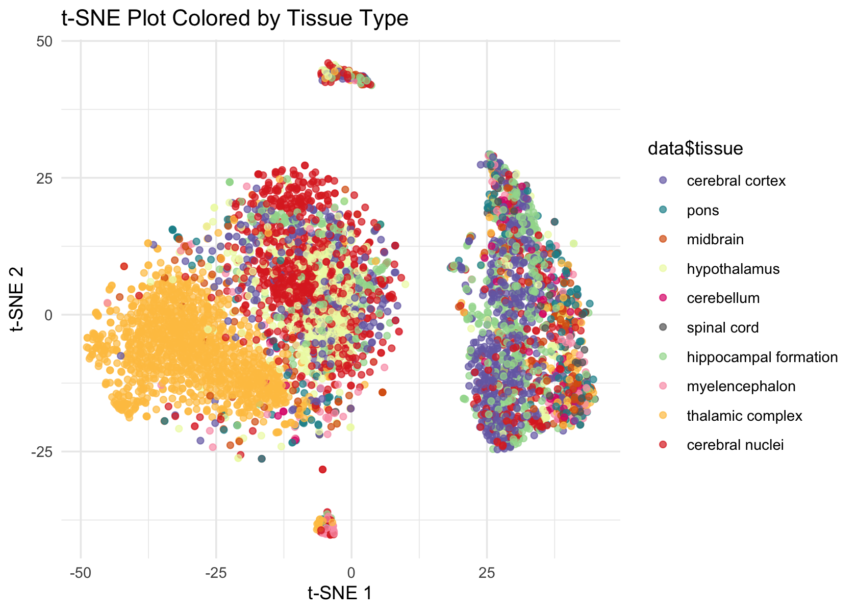

Version	Author	Date
7a353a3	junmingguan	2024-11-09


# colors <- brewer.pal(length(unique(regions)), "Set1")
# ggplot(Embeddings(data$tSNE) , aes(x = TSNE_1, y = TSNE_2, color = regions)) +
#   geom_point(alpha = 0.7) +
#   labs(title = "t-SNE Plot Colored by Tissue Type", x = "t-SNE 1", y = "t-SNE 2") +
#   theme_minimal() +
#   scale_color_manual(values = colors)

# colors <- brewer.pal(length(unique(data$cluster_id)), "Paired")
colors <-  c('#756bb1', '#1c9099', '#d95f0e', '#edf8b1', '#dd1c77', '#636363', '#a1d99b')
ggplot(Embeddings(data$tSNE) , aes(x = TSNE_1, y = TSNE_2, color = data$cluster_id)) +
  geom_point(alpha = 0.7) +
  labs(title = "t-SNE Plot Colored by Cluster", x = "t-SNE 1", y = "t-SNE 2") +
  theme_minimal() +
  scale_color_manual(values = colors)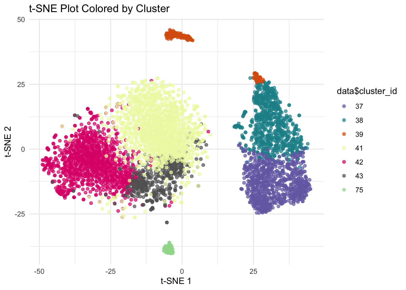

Version	Author	Date
7a353a3	junmingguan	2024-11-09

UMAP

# colors <- brewer.pal(length(unique(data$tissue)), "Paired")
colors <-  c('#756bb1', '#1c9099', '#d95f0e', '#edf8b1', '#dd1c77', '#636363', '#a1d99b', '#fa9fb5', '#fec44f', '#de2d26')
ggplot(Embeddings(data$UMAP) , aes(x = UMAP_1, y = UMAP_2, color = data$tissue)) +
  geom_point(alpha = 0.7) +
  labs(title = "UMAP Plot Colored by Tissue Type", x = "UMAP 1", y = "UMAP 2") +
  theme_minimal() +
  scale_color_manual(values = colors)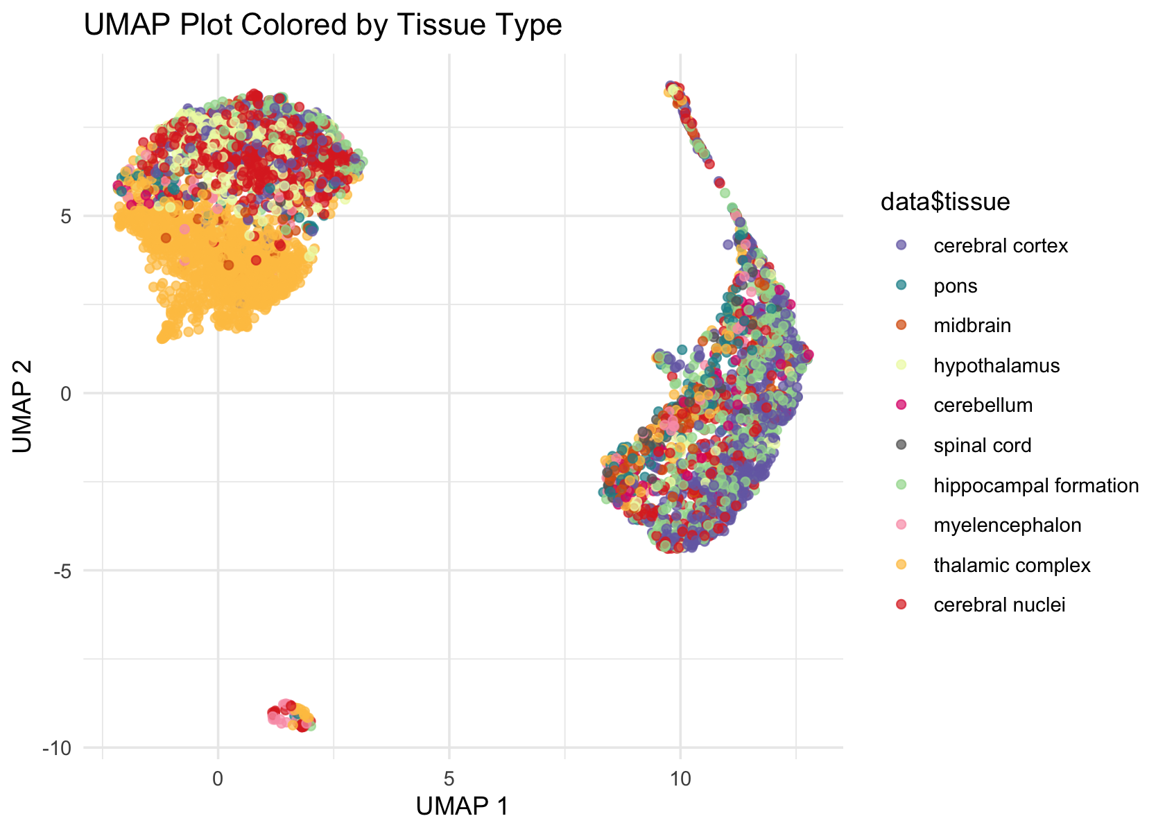

Version	Author	Date
7a353a3	junmingguan	2024-11-09


# ggplot(Embeddings(data$UMAP) , aes(x = UMAP_1, y = UMAP_2, color = regions)) +
#   geom_point(alpha = 0.7) +
#   labs(title = "UMAP Plot Colored by Tissue Type", x = "UMAP 1", y = "UMAP 2") +
#   theme_minimal() +
#   scale_color_manual(values = rainbow(length(unique(regions))))

# colors <- brewer.pal(length(unique(data$cluster_id)), "Paired")
colors <-  c('#756bb1', '#1c9099', '#d95f0e', '#edf8b1', '#dd1c77', '#636363', '#a1d99b')
ggplot(Embeddings(data$UMAP) , aes(x = UMAP_1, y = UMAP_2, color = data$cluster_id)) +
  geom_point(alpha = 0.7) +
  labs(title = "UMAP Plot Colored by Cluster", x = "UMAP 1", y = "UMAP 2") +
  theme_minimal() +
  scale_color_manual(values = colors)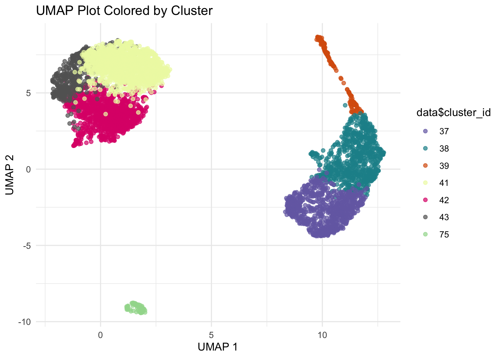

Version	Author	Date
7a353a3	junmingguan	2024-11-09

Flashier

NMF

Redefine subcluster ids so that the hierarchical structure is clearer

# M <- table(data$subcluster_id, data$cluster_id)
# M
subcluster_id <- as.vector(data$subcluster_id)
subcluster_id[subcluster_id == '3033'] <- '37.1'
subcluster_id[subcluster_id == '3035'] <- '37.2'
subcluster_id[subcluster_id == '3036'] <- '37.3'
subcluster_id[subcluster_id == '3037'] <- '37.4'
subcluster_id[subcluster_id == '3038'] <- '37.5'

subcluster_id[subcluster_id == '3030'] <- '38.1'
subcluster_id[subcluster_id == '3031'] <- '38.2'
subcluster_id[subcluster_id == '3032'] <- '38.3'
subcluster_id[subcluster_id == '3034'] <- '38.4'

subcluster_id[subcluster_id == '3027'] <- '39.1'
subcluster_id[subcluster_id == '3028'] <- '39.2'
subcluster_id[subcluster_id == '3029'] <- '39.3'

subcluster_id[subcluster_id == '3014'] <- '41.1'
subcluster_id[subcluster_id == '3015'] <- '42.2'

subcluster_id[subcluster_id == '3007'] <- '42.1'
subcluster_id[subcluster_id == '3008'] <- '42.2'
subcluster_id[subcluster_id == '3009'] <- '42.3'
subcluster_id[subcluster_id == '3010'] <- '42.4'

subcluster_id[subcluster_id == '3006'] <- '43.1'

subcluster_id[subcluster_id == '3195'] <- '75.1'
subcluster_id[subcluster_id == '3196'] <- '75.2'
subcluster_id <- factor(subcluster_id)

flash_plot_scree(flashier_fit)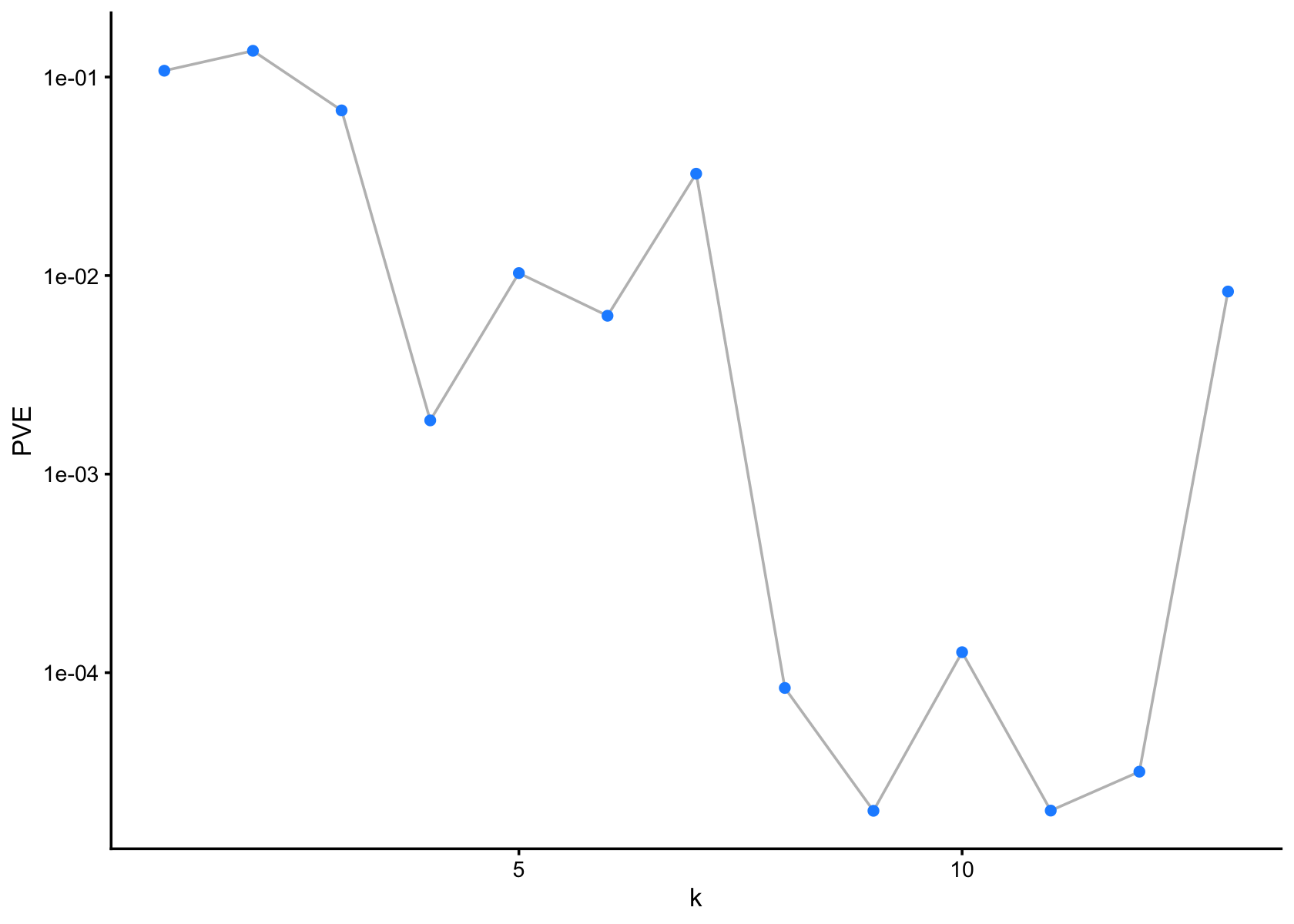

Version	Author	Date
7a353a3	junmingguan	2024-11-09



plot(flashier_fit, 
     plot_type = "heatmap",
     pm_which = "loadings", 
     pm_groups = data$cluster_id,
     gap = 25)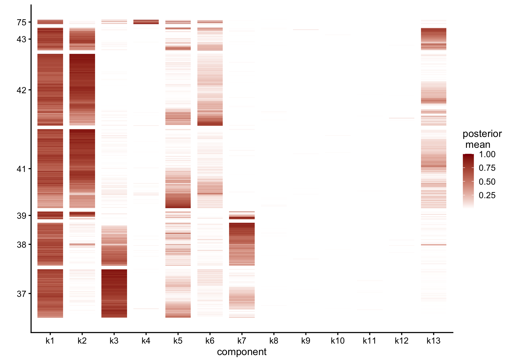

Version	Author	Date
7a353a3	junmingguan	2024-11-09


plot(flashier_fit, 
     plot_type = "histogram",
     pm_which = "loadings", 
     pm_groups = data$cluster_id,
     bins = 25)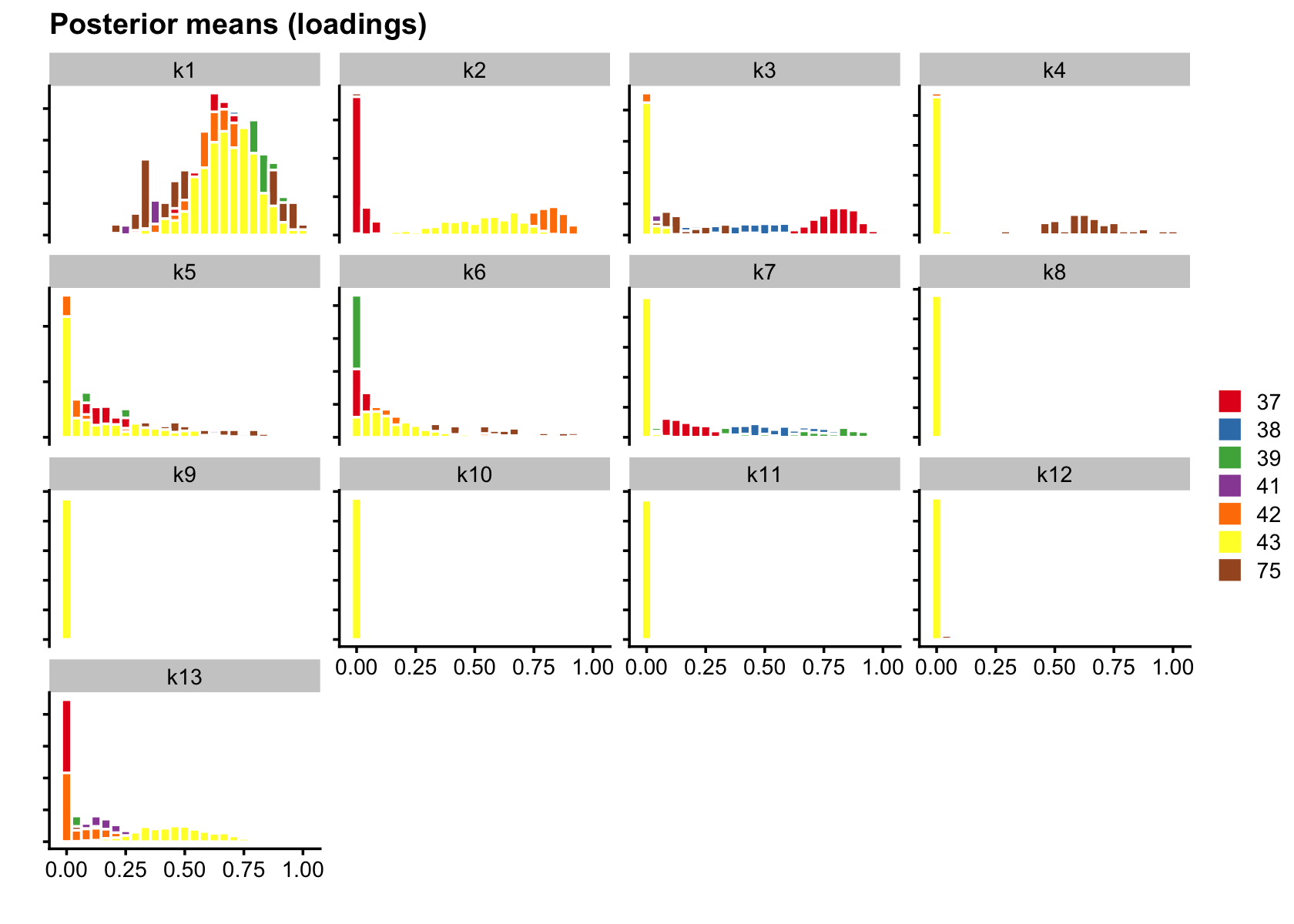

Version	Author	Date
7a353a3	junmingguan	2024-11-09

plot(flashier_fit, 
     plot_type = "structure",
     pm_which = "loadings", 
     pm_groups = data$cluster_id,
     bins = 30, gap = 70)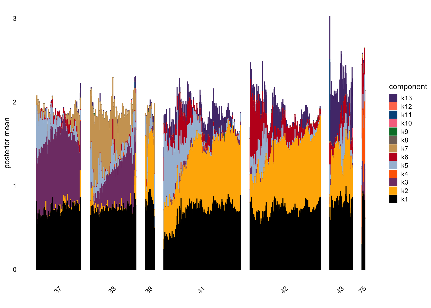

Version	Author	Date
7a353a3	junmingguan	2024-11-09


plot(flashier_fit, 
     plot_type = "structure",
     pm_which = "loadings", 
     pm_groups = subcluster_id,
     bins = 60, gap = 100)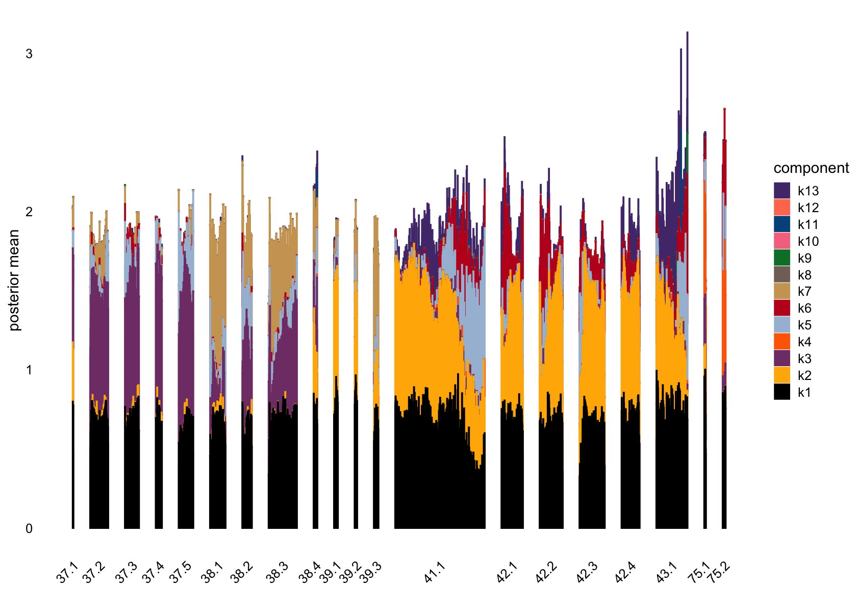

Version	Author	Date
7a353a3	junmingguan	2024-11-09

vals <- ldf(flashier_fit,type="m")
ncells <- colSums(vals$L>0.1)
ncells
#  [1] 4720 3101 1557   79 2059 1640 1281    1    5    1    4    2 1800

Several factors are load on only a small number of cells.

Removing those factors from the structure plots:

plot(flashier_fit, 
     kset = which(ncells > 5),
     plot_type = "structure",
     pm_which = "loadings", 
     pm_groups = data$cluster_id,
     bins = 30, gap = 70)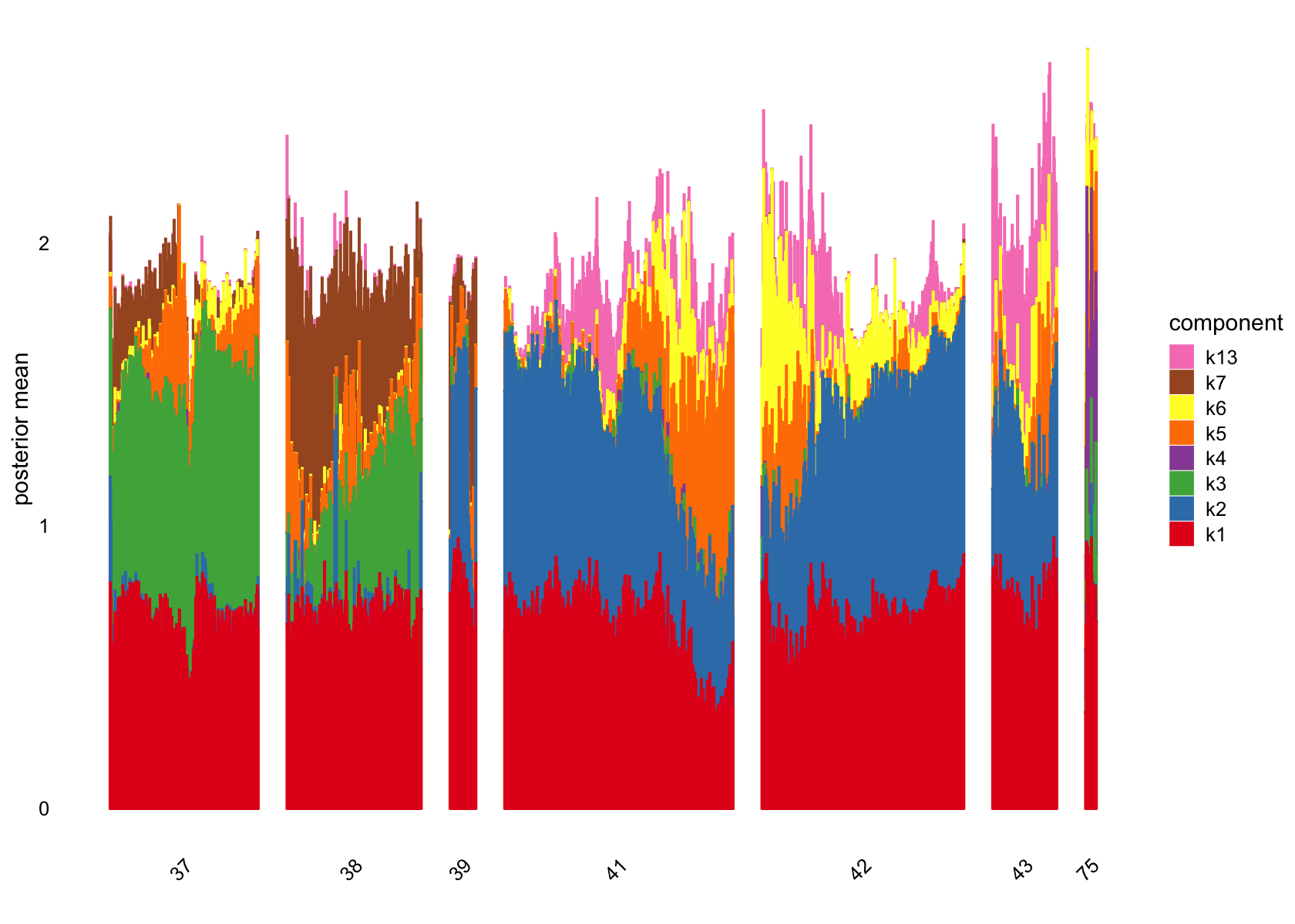

Version	Author	Date
7a353a3	junmingguan	2024-11-09


plot(flashier_fit, 
     kset = which(ncells > 5),
     plot_type = "structure",
     pm_which = "loadings", 
     pm_groups = subcluster_id,
     bins = 60, gap = 100)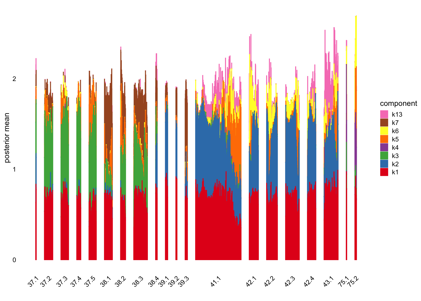

Version	Author	Date
7a353a3	junmingguan	2024-11-09

Showing those factors in the structure plots:

plot(flashier_fit, 
     kset = which(ncells <= 5),
     plot_type = "structure",
     pm_which = "loadings", 
     pm_groups = data$cluster_id,
     bins = 30, gap = 70)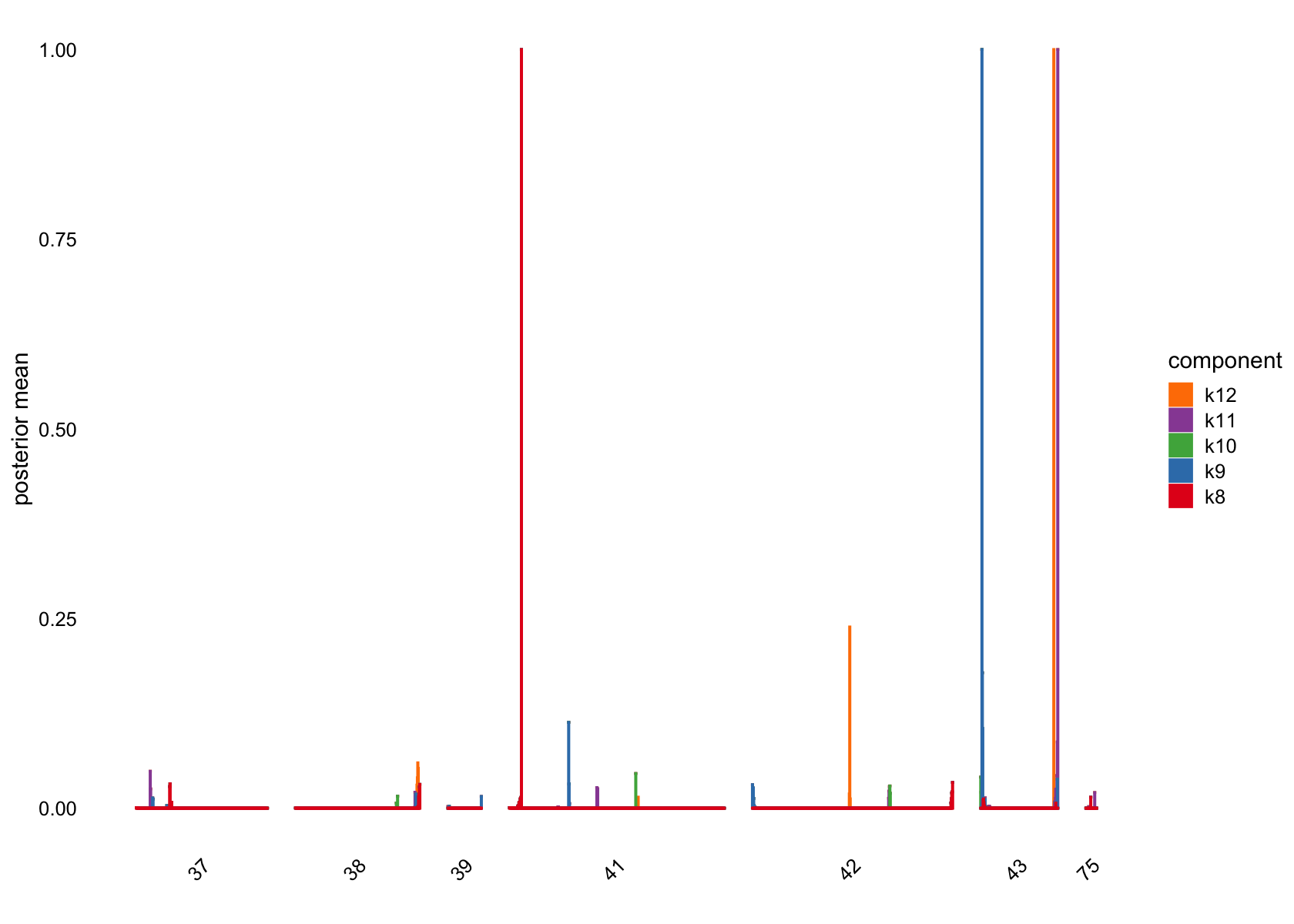

Version	Author	Date
7a353a3	junmingguan	2024-11-09


plot(flashier_fit, 
     kset = which(ncells <= 5),
     plot_type = "structure",
     pm_which = "loadings", 
     pm_groups = subcluster_id,
     bins = 60, gap = 100)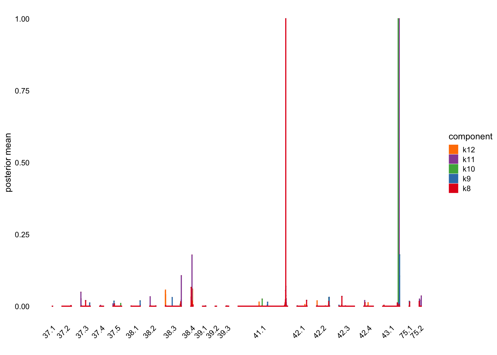

Version	Author	Date
7a353a3	junmingguan	2024-11-09

Top 5 driving genes for factors that are loading on a small number of cells

F <- with(vals, F %*% diag(D))
rownames(F) <- homo_sapien_geno_info$Symbol[match(rownames(F), 
                                            homo_sapien_geno_info$Ensembl)]
head(sort(F[,8], decreasing = TRUE), n = 16)


top_genes <- apply(F, 2, order, decreasing = TRUE)[1:5, which(ncells<=5)]
top_genes <- rownames(flashier_fit$F_pm)[top_genes]

plot(flashier_fit,
     plot_type = "heatmap",
     pm_which = "factors",
     pm_subset = top_genes,
     pm_groups = factor(top_genes),
     kset = which(ncells<=5),
     gap = 0.5)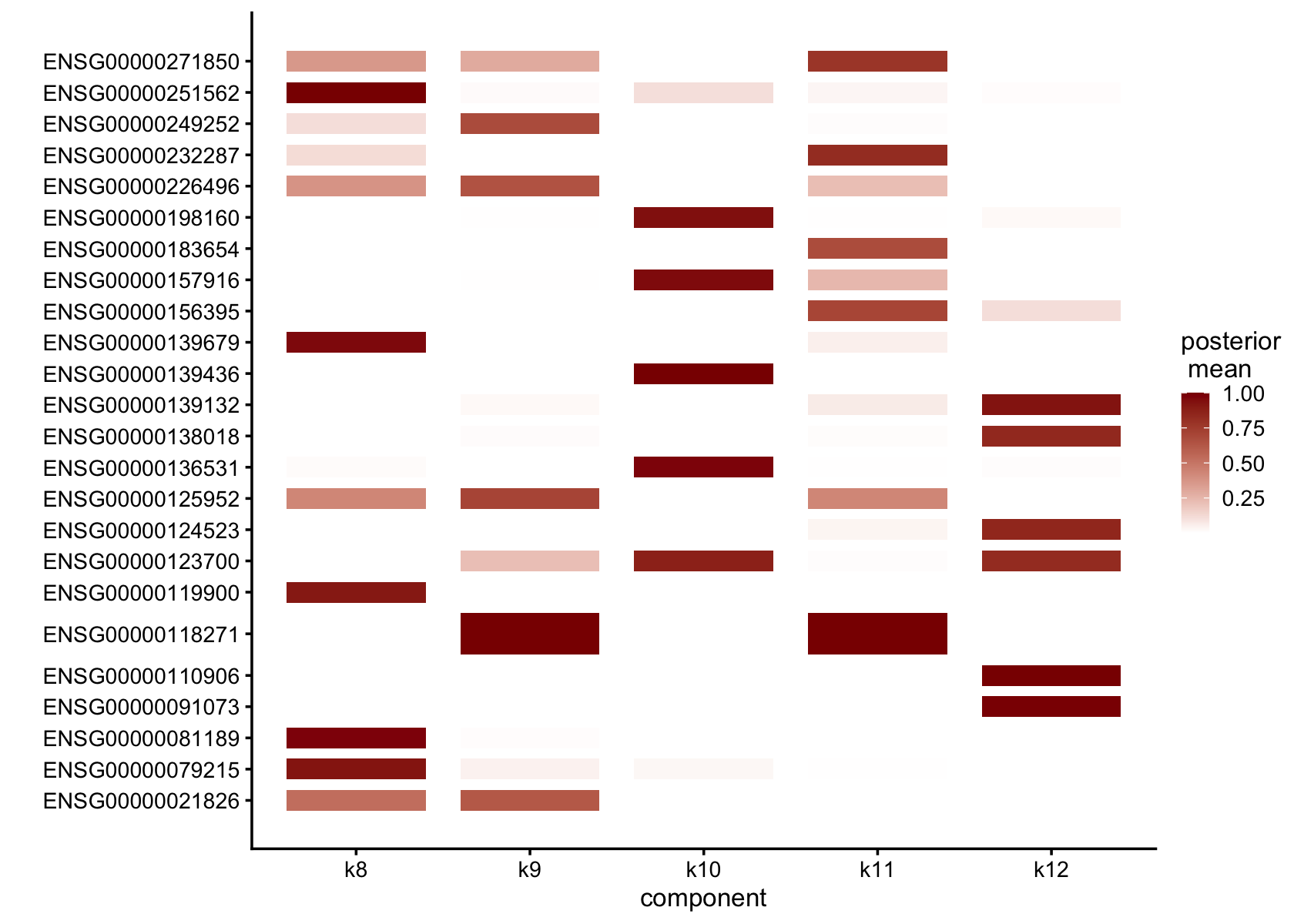

Plot of mean shifted log expression vs. change for factor 8, with top 5 genes (by largest increase)

plot(flashier_fit,
     plot_type = "scatter",
     pm_which = "factors",
     kset = 8,
     labels = TRUE,
     n_labels = 5,
     label_size = 2.5) +
  labs(x = "increase in shifted log expression",
       y = "mean shifted log expression")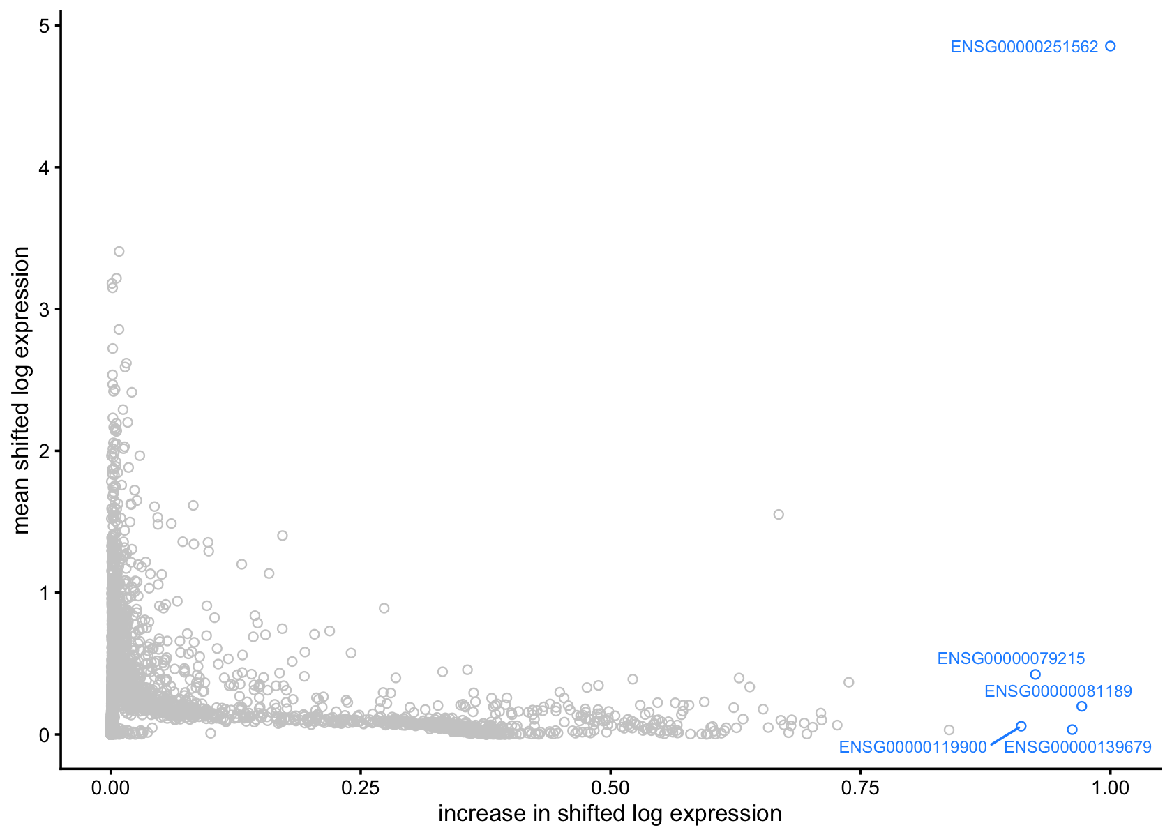

Symbols of top 5 driving genes for

top5_genes_factor_8 <- 
  sort(with(vals, F %*% diag(D))[, 8], decreasing = TRUE) %>% 
  head(., 5) %>%
  names()
homo_sapien_geno_info[match(top5_genes_factor_8, homo_sapien_geno_info$Ensembl),
                      c('Symbol', 'Ensembl')]
#       Symbol         Ensembl
# 22566 MALAT1 ENSG00000251562
# 3394   MEF2C ENSG00000081189
# 7946   LPAR6 ENSG00000139679
# 5159  SLC1A3 ENSG00000079215
# 14744 OGFRL1 ENSG00000119900

For factor 8

MALAT1 (Metastasis-Associated Lung Adenocarcinoma Transcript 1)
- Long non-coding RNA (lncRNA)
MEF2C (Myocyte Enhancer Factor 2C)
- Transcription factor
LPAR6 (Lysophosphatidic Acid Receptor 6)
- G-protein-coupled receptor
SLC1A3 (Solute Carrier Family 1 Member 3)
- Glutamate transporter
OGFRL1 (Opioid Growth Factor Receptor-Like 1)
- Putative receptor

From chatGPT

Loadings on UMAP by factor

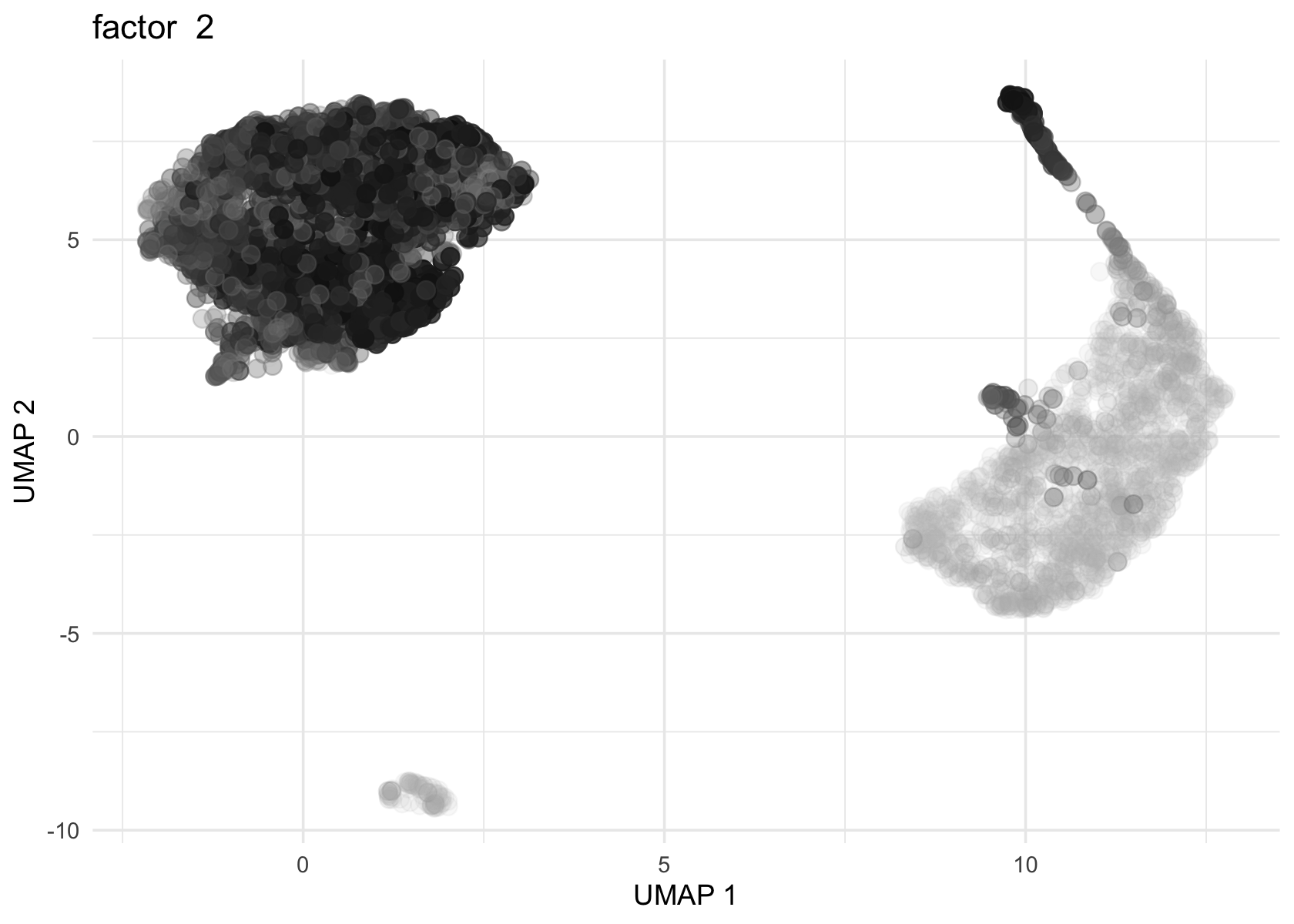
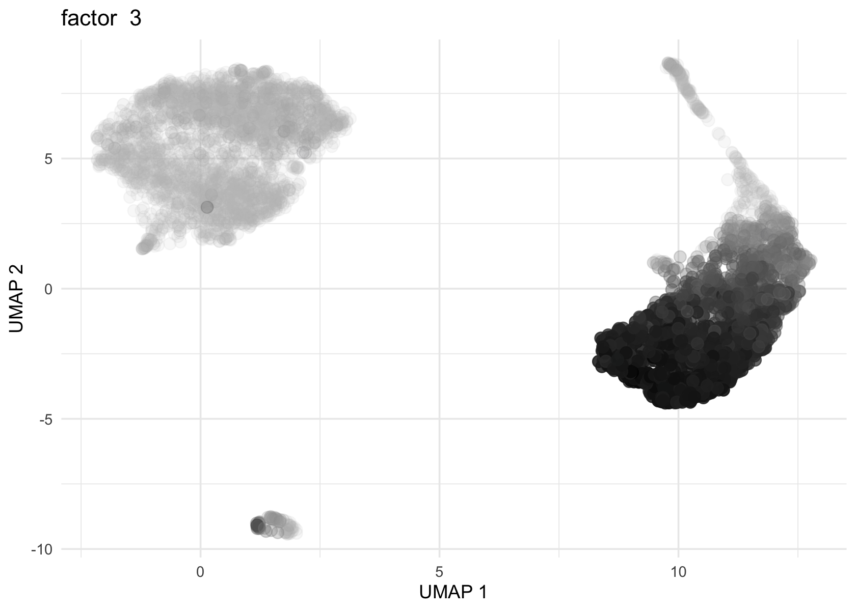
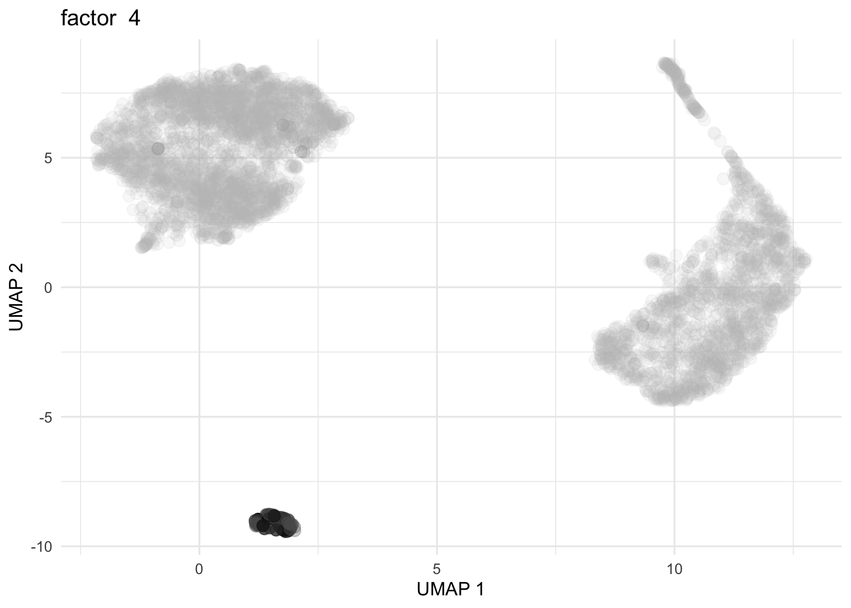
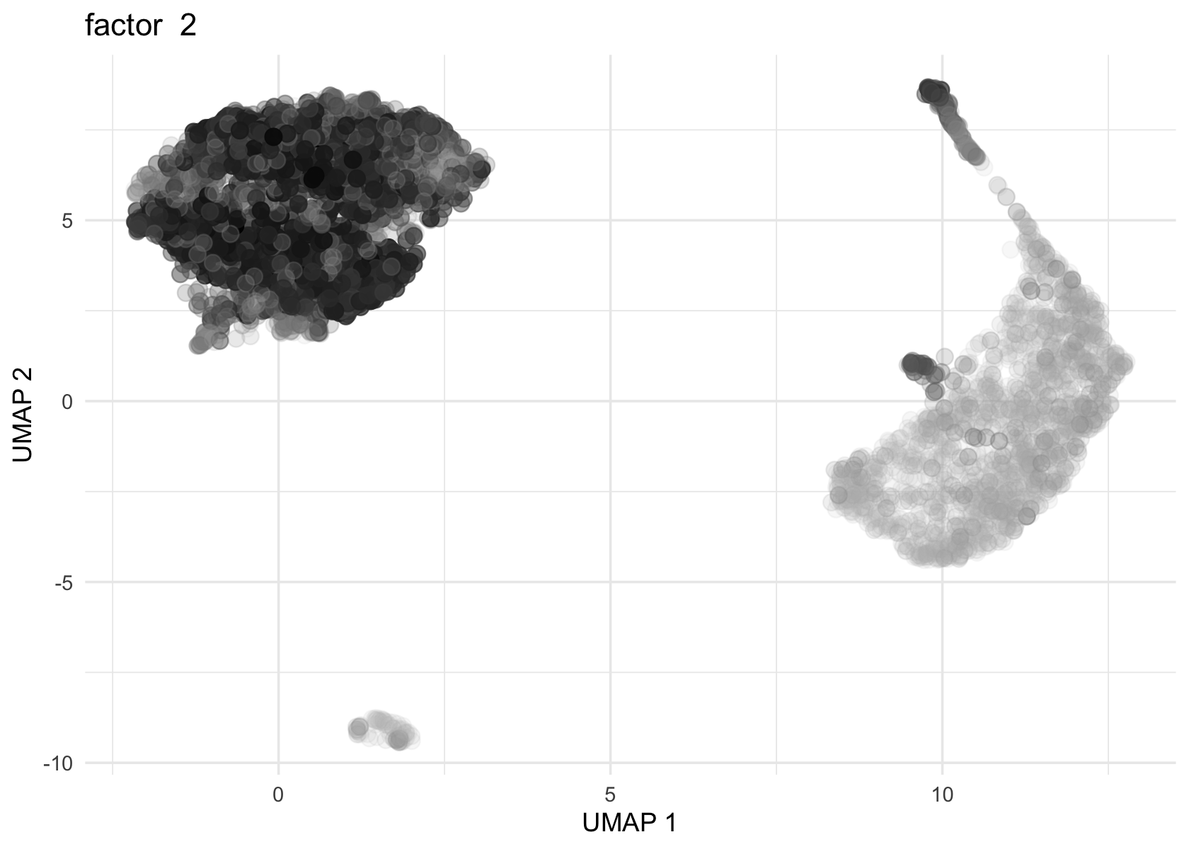
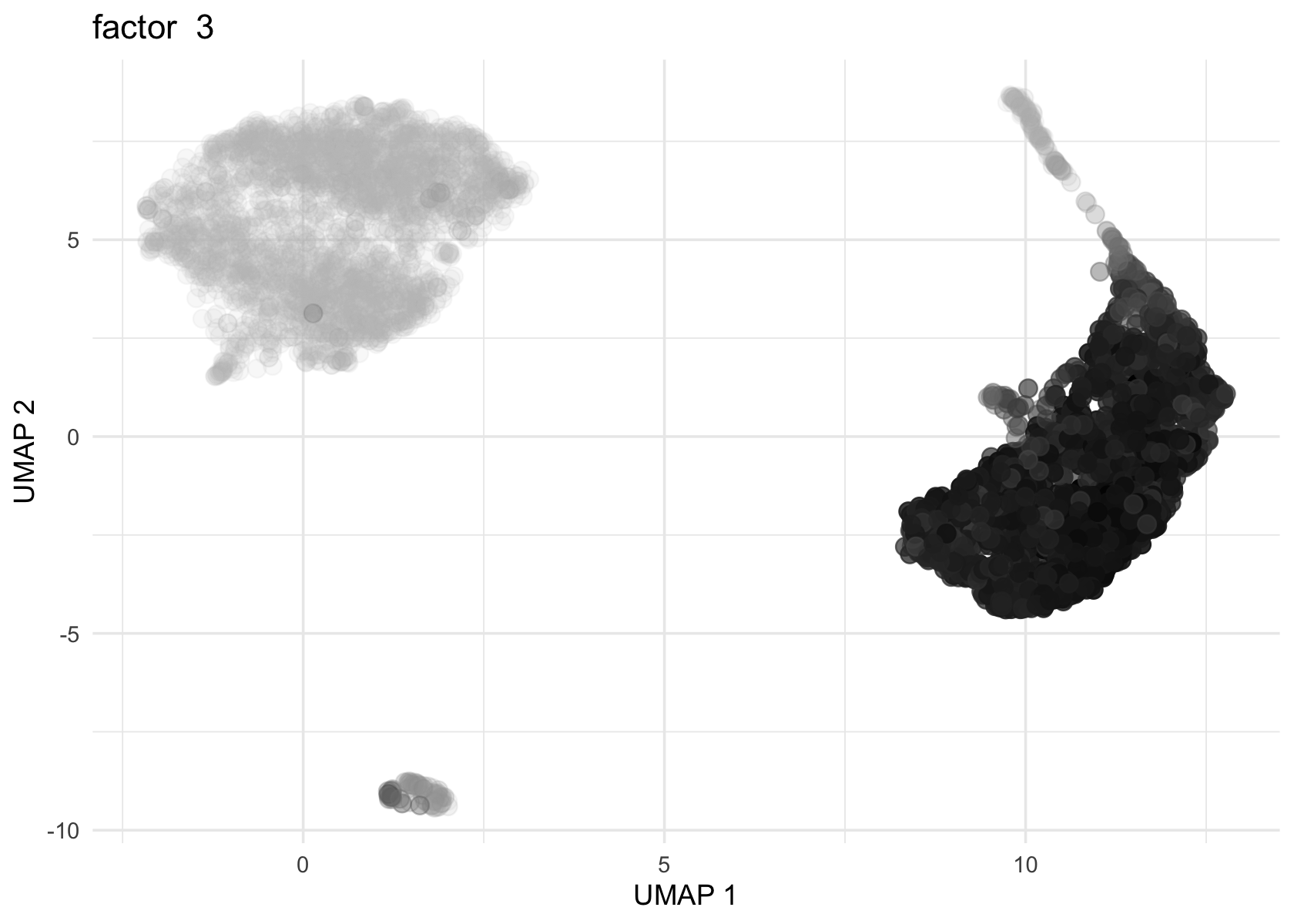
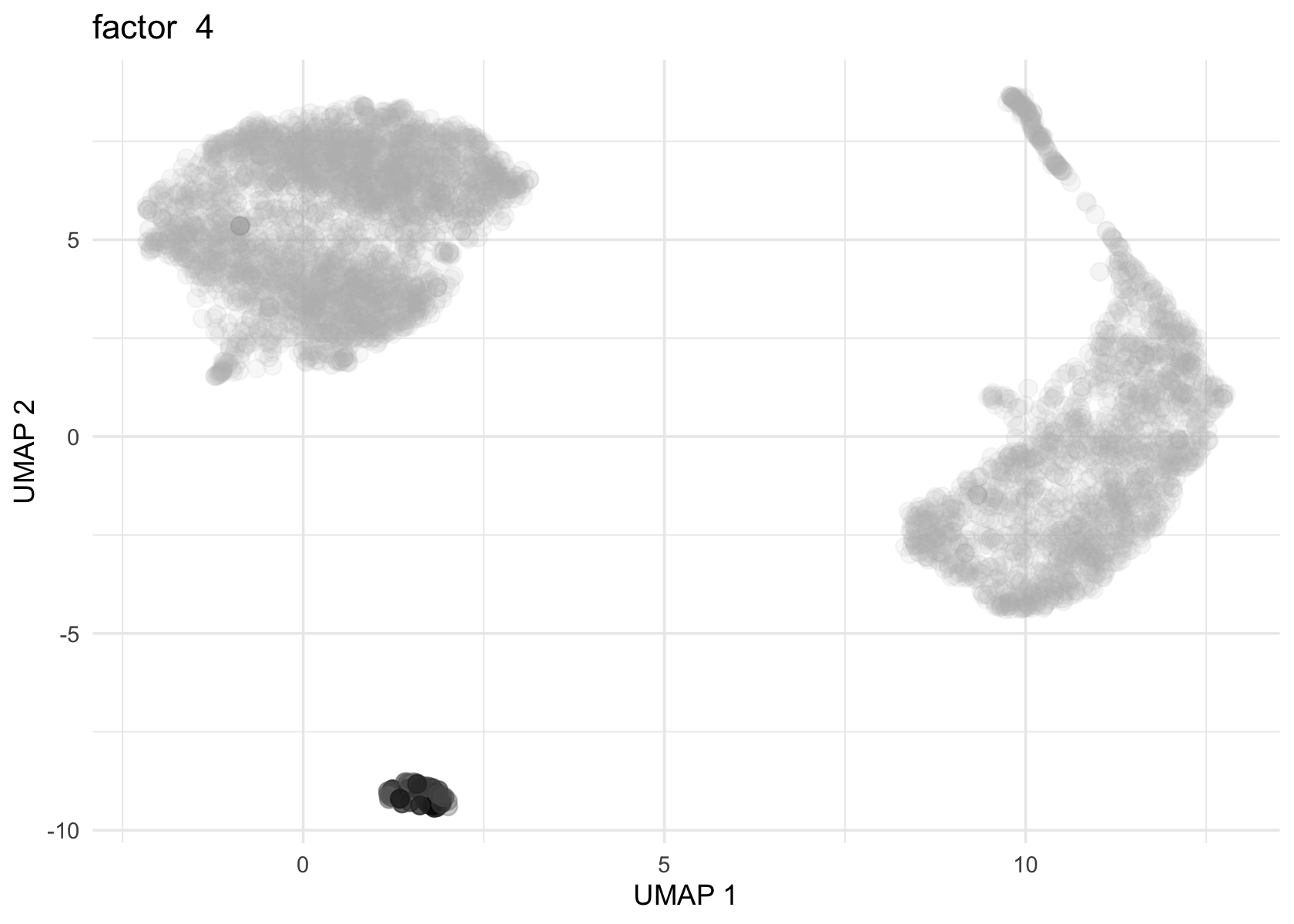
Factor 2, 3 and 4 are heavily loaded, whereas factor 8 and 9 are loaded on a single cell.

umap <- Embeddings(data$UMAP)
source('../code/plot_loadings_on_umap.R')

for (f in c(2, 3, 4, 8, 9)) {
  loading <- vals$L[, f]
  p <- plot_loadings_on_umap(umap, loading, f)
  print(p)
}

Version	Author	Date
47fa791	junmingguan	2024-11-17

Version	Author	Date
47fa791	junmingguan	2024-11-17

Version	Author	Date
47fa791	junmingguan	2024-11-17

Version	Author	Date
47fa791	junmingguan	2024-11-17

Version	Author	Date
47fa791	junmingguan	2024-11-17

Semi-NMF

flash_plot_scree(flashier_fit_semi)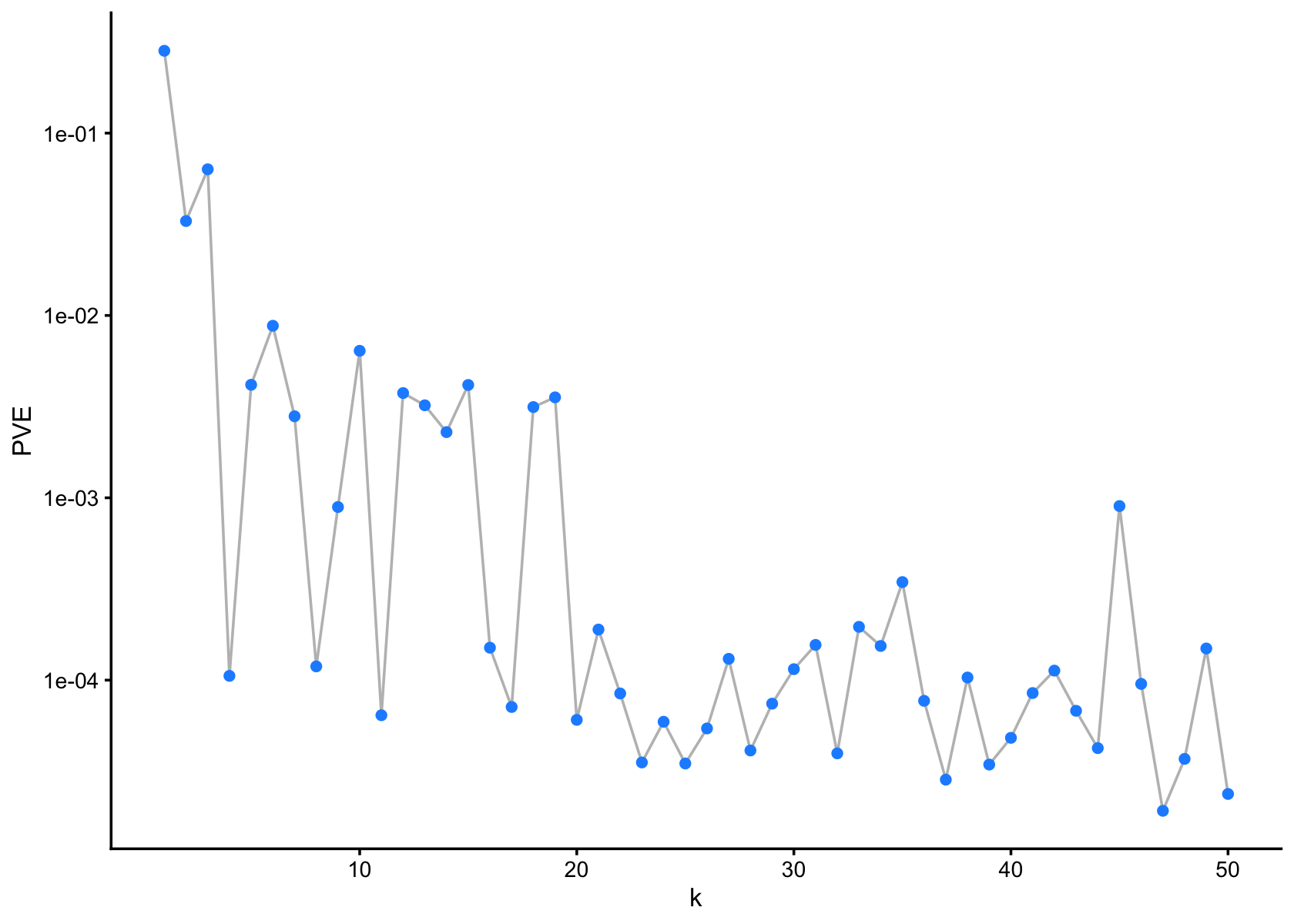

Version	Author	Date
7a353a3	junmingguan	2024-11-09



plot(flashier_fit_semi, 
     plot_type = "heatmap",
     pm_which = "loadings", 
     pm_groups = data$cluster_id,
     gap = 25)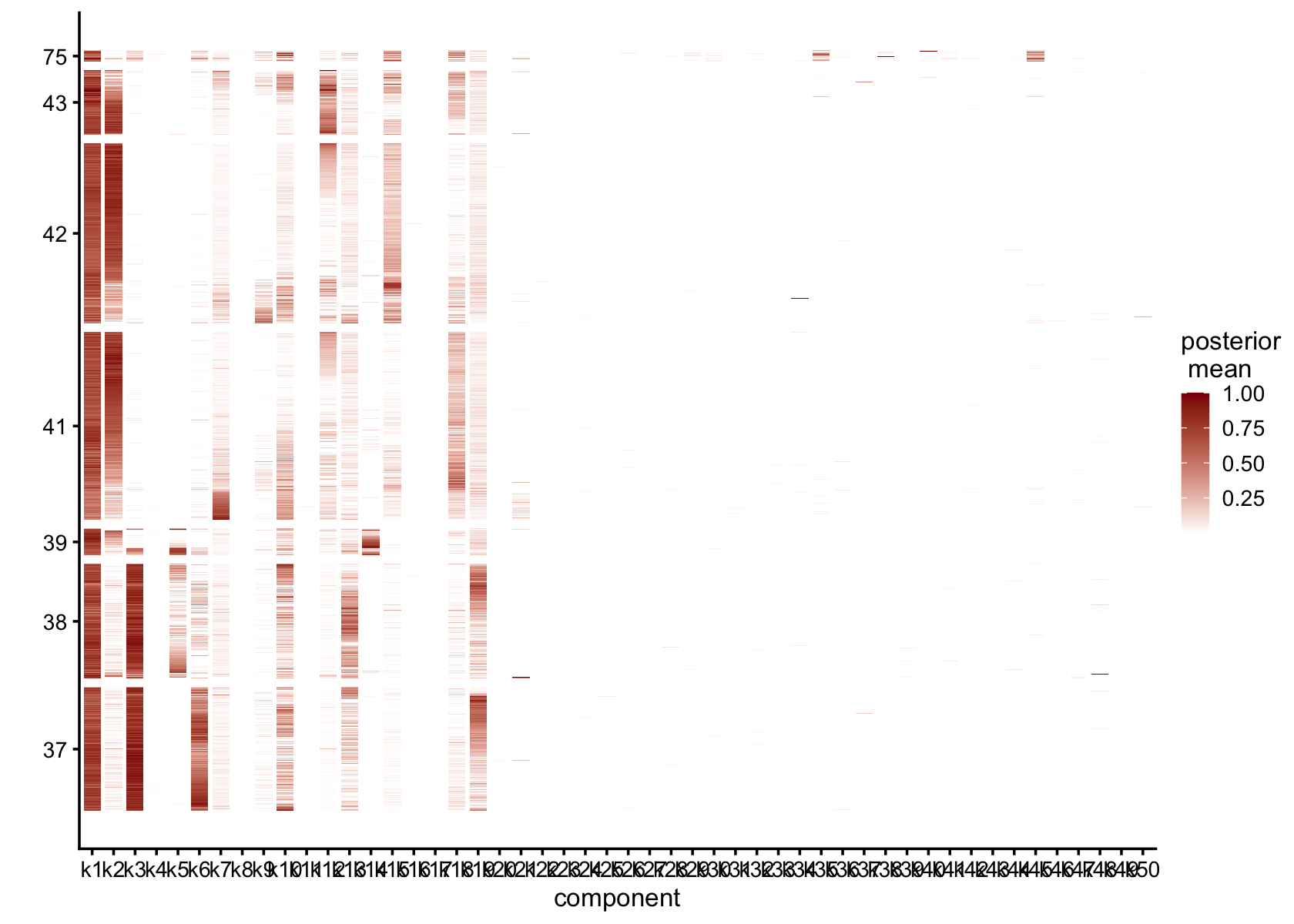

Version	Author	Date
7a353a3	junmingguan	2024-11-09


plot(flashier_fit_semi, 
     plot_type = "histogram",
     pm_which = "loadings", 
     pm_groups = data$cluster_id,
     bins = 25)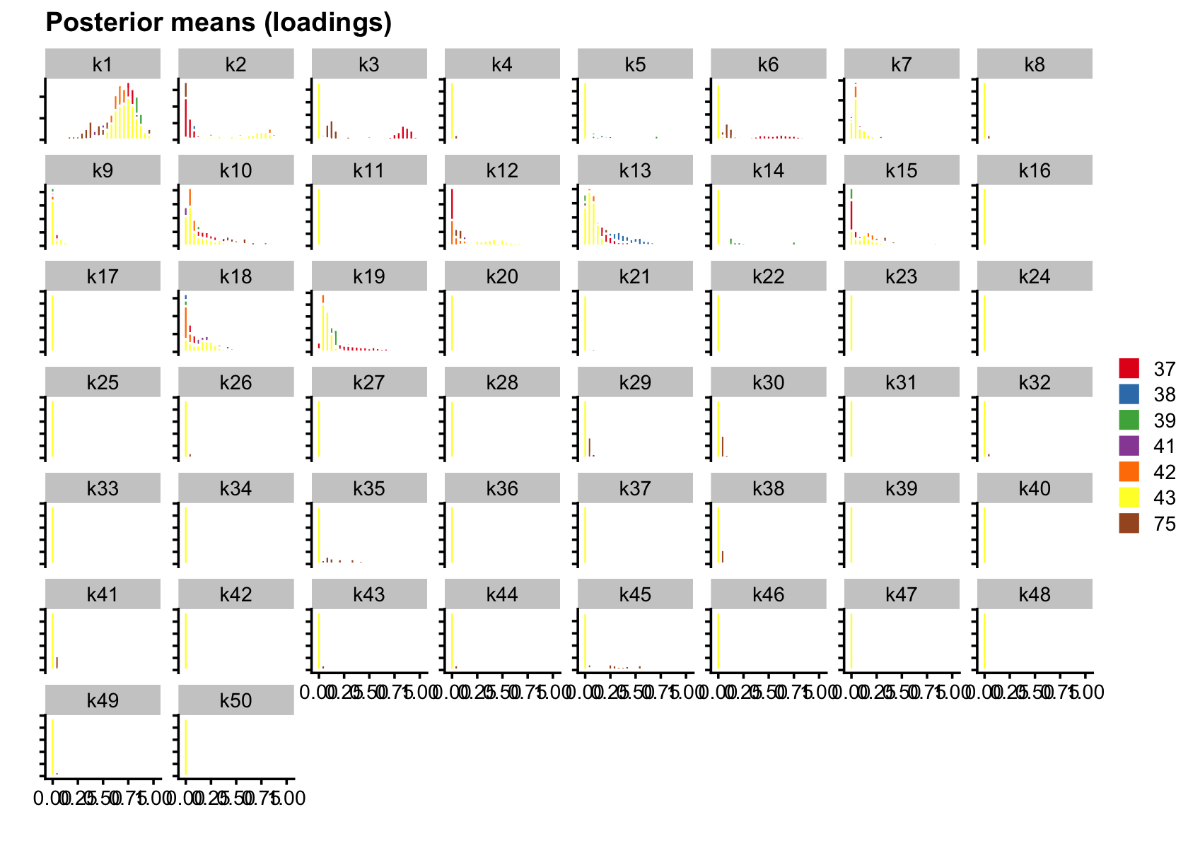

Version	Author	Date
7a353a3	junmingguan	2024-11-09

plot(flashier_fit_semi, 
     plot_type = "structure",
     pm_which = "loadings", 
     pm_groups = data$cluster_id,
     bins = 30, gap = 70)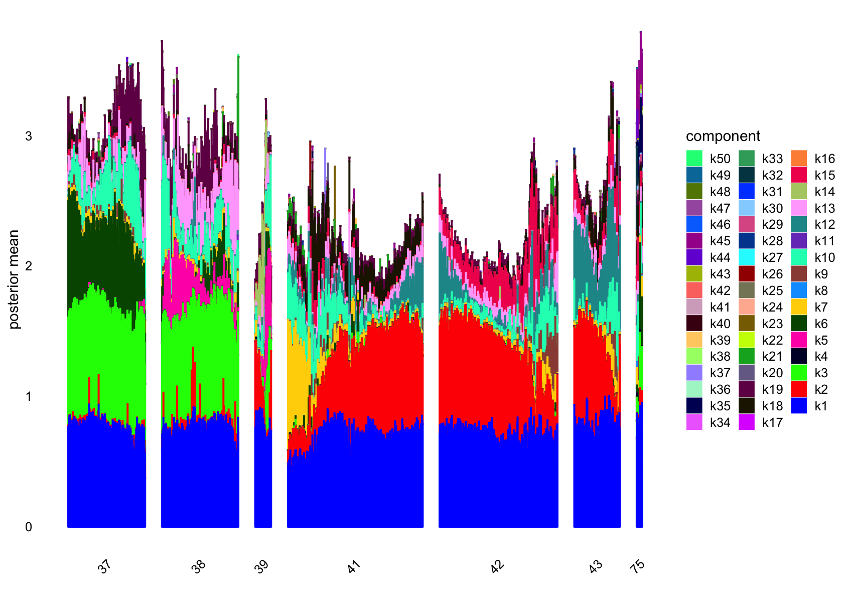

Version	Author	Date
7a353a3	junmingguan	2024-11-09


plot(flashier_fit_semi, 
     plot_type = "structure",
     pm_which = "loadings", 
     pm_groups = subcluster_id,
     bins = 60, gap = 100)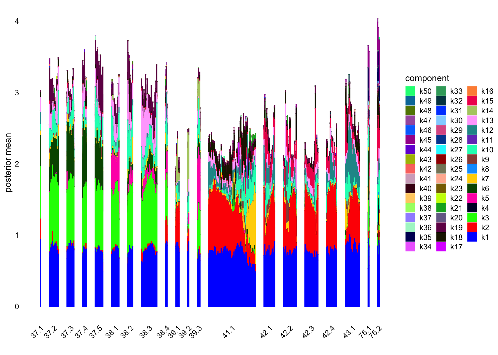

Version	Author	Date
7a353a3	junmingguan	2024-11-09

vals_semi <- ldf(flashier_fit_semi, type="m")
ncells_semi <- colSums(vals_semi$L>0.1)
ncells_semi
#  [1] 4720 3074 1702   72  558 1205 2239    1  308 1669    1 1497 1704  181 1584
# [16]    1    1 1831 1900    3  126    1    2    1    3    1    2    5    1    6
# [31]    1    2    1    1    4    1    1    5    1    1    4    2    1    4    2
# [46]    2    2    3    1    3

Several factors are load on only a small number of cells.

Removing those factors from the structure plots:

plot(flashier_fit_semi, 
     kset = which(ncells_semi > 5),
     plot_type = "structure",
     pm_which = "loadings", 
     pm_groups = data$cluster_id,
     bins = 30, gap = 70)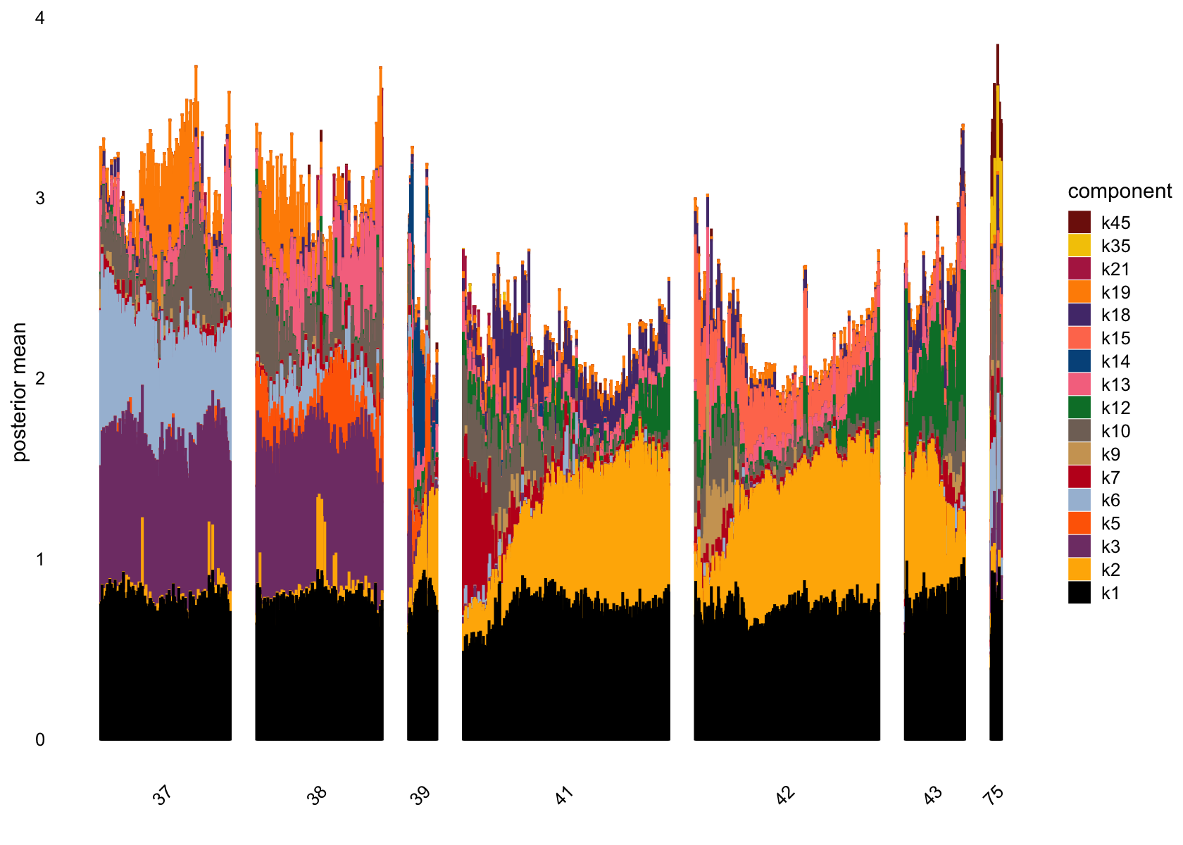

Version	Author	Date
7a353a3	junmingguan	2024-11-09


plot(flashier_fit_semi, 
     kset = which(ncells_semi > 5),
     plot_type = "structure",
     pm_which = "loadings", 
     pm_groups = subcluster_id,
     bins = 60, gap = 100)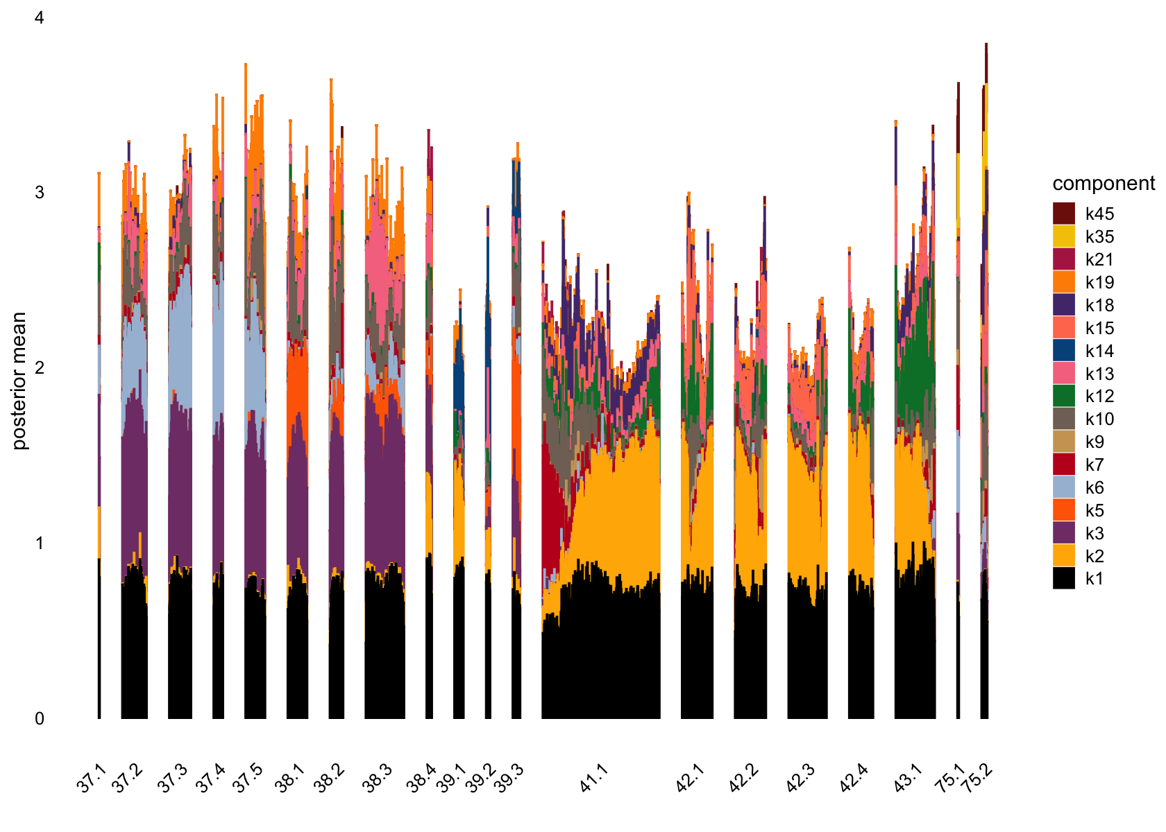

Version	Author	Date
7a353a3	junmingguan	2024-11-09

Showing factors that are only loaded on a small number of cells:

plot(flashier_fit_semi, 
     kset = which(ncells_semi <= 5),
     plot_type = "structure",
     pm_which = "loadings", 
     pm_groups = data$cluster_id,
     bins = 30, gap = 70)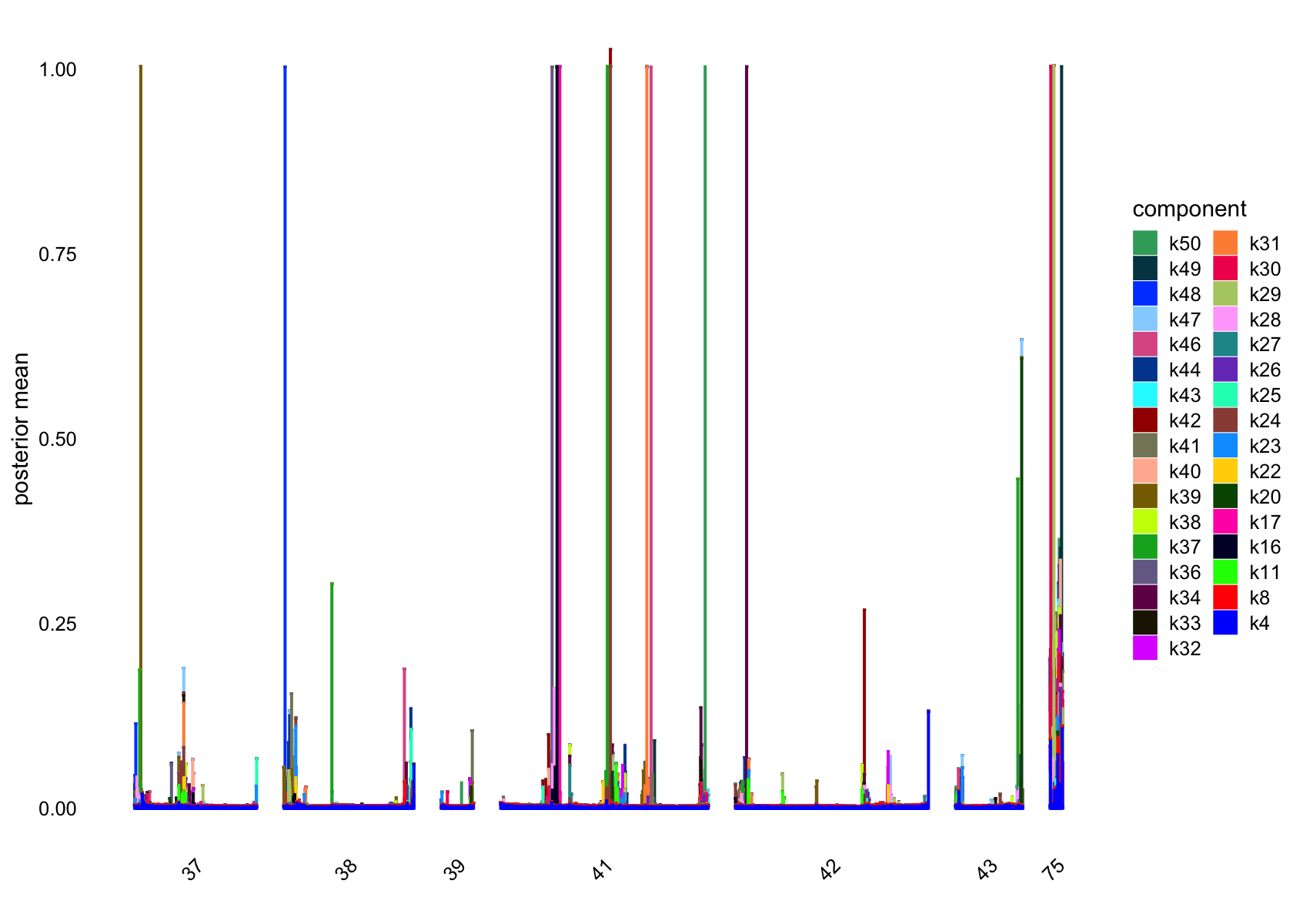

Version	Author	Date
7a353a3	junmingguan	2024-11-09


plot(flashier_fit_semi, 
     kset = which(ncells_semi <= 5),
     plot_type = "structure",
     pm_which = "loadings", 
     pm_groups = subcluster_id,
     bins = 60, gap = 100)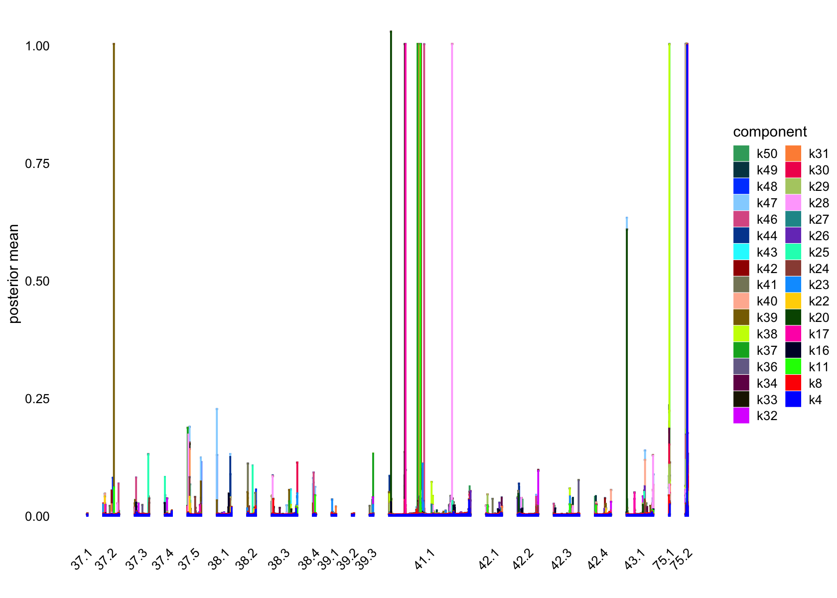

Version	Author	Date
7a353a3	junmingguan	2024-11-09

Top 5 driving genes for factors that are loading on a small number of cells

F <- with(vals_semi, F %*% diag(D))
rownames(F) <- homo_sapien_geno_info$Symbol[match(rownames(F), 
                                            homo_sapien_geno_info$Ensembl)]
head(sort(F[,8], decreasing = TRUE), n = 16)
# top_genes <- apply(F, 2, order, decreasing = TRUE)[1:5, c(8, 11)]
# top_genes <- rownames(flashier_fit_semi$F_pm)[top_genes]
# 
# plot(flashier_fit_semi,
#      plot_type = "heatmap",
#      pm_which = "factors",
#      pm_subset = top_genes,
#      pm_groups = factor(top_genes),
#      kset = c(8, 11),
#      gap = 0.5)

Plot of mean shifted log expression vs. change for factor 8, with top 5 genes (by largest increase)

plot(flashier_fit_semi,
     plot_type = "scatter",
     pm_which = "factors",
     kset = c(8, 11, 16),
     labels = TRUE,
     n_labels = 5,
     label_size = 2.5) +
  labs(x = "increase in shifted log expression",
       y = "mean shifted log expression")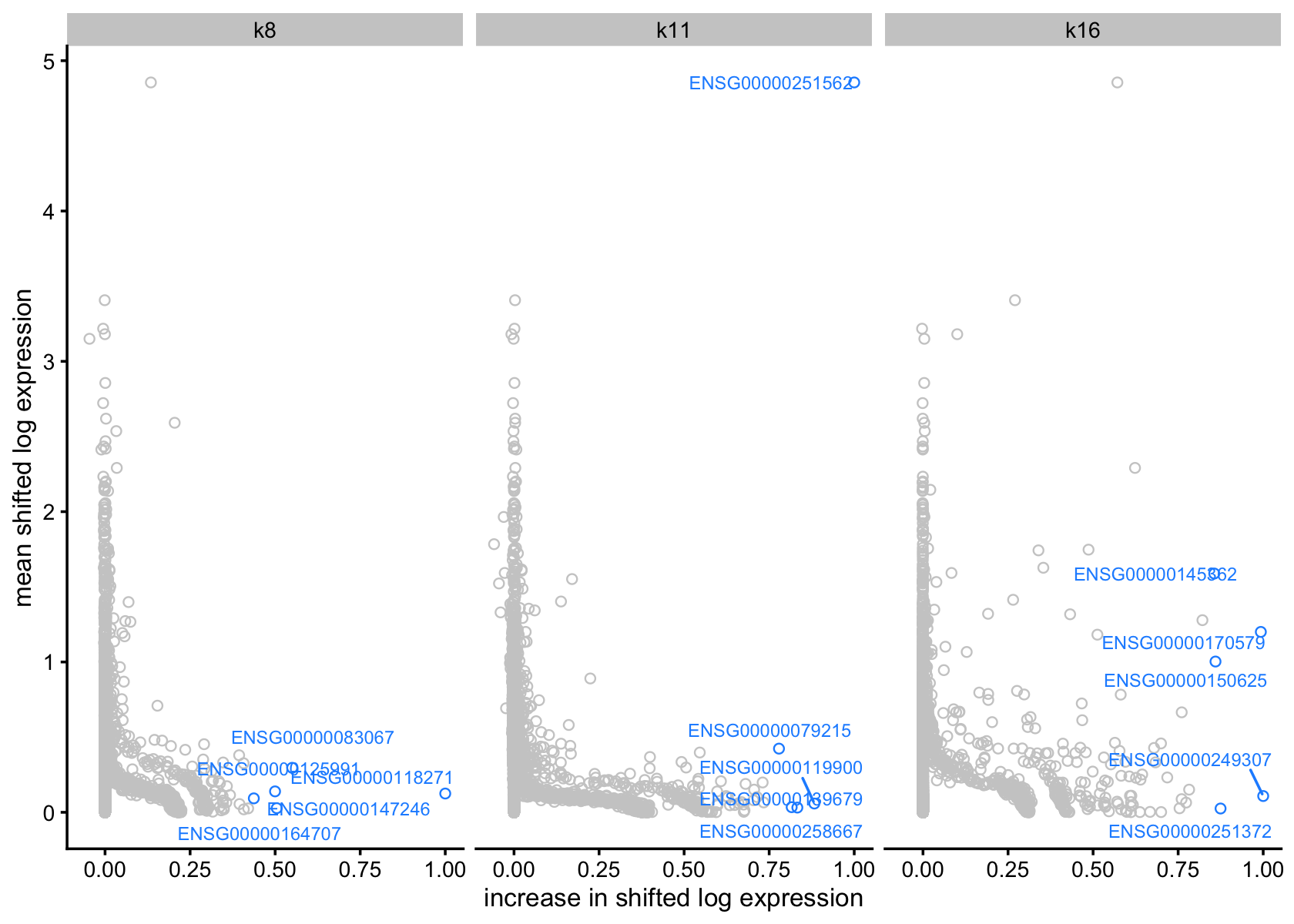

Symbols of top 5 driving genes for factor 11

top5_genes_factor_11 <- 
  sort(with(vals_semi, F %*% diag(D))[, 11], decreasing = TRUE) %>% 
  head(., 5) %>%
  names()
homo_sapien_geno_info[match(top5_genes_factor_11, homo_sapien_geno_info$Ensembl),
                      c('Symbol', 'Ensembl')]
#          Symbol         Ensembl
# 22566    MALAT1 ENSG00000251562
# 14744    OGFRL1 ENSG00000119900
# 43448 HIF1A-AS3 ENSG00000258667
# 7946      LPAR6 ENSG00000139679
# 5159     SLC1A3 ENSG00000079215

For factor 8

MALAT1 (Metastasis-Associated Lung Adenocarcinoma Transcript 1)
- Long non-coding RNA (lncRNA)
OGFRL1 (Opioid Growth Factor Receptor-Like 1)
- Putative receptor
HIF1A-AS3
- Associated with hypoxia regulation and cancer biology
- Long non-coding RNA (lncRNA)
LPAR6 (Lysophosphatidic Acid Receptor 6)
- G-protein-coupled receptor
SLC1A3 (Solute Carrier Family 1 Member 3)
- Glutamate transporter From chatGPT

Loadings on UMAP by factor

Factor 2 and 3 are heavily loaded, whereas factor 4, 8 and 11 are loaded on a few cells.

umap <- Embeddings(data$UMAP)
source('../code/plot_loadings_on_umap.R')

for (f in c(2, 3, 4, 8, 11)) {
  loading <- vals_semi$L[, f]
  p <- plot_loadings_on_umap(umap, loading, f)
  print(p)
}

Version	Author	Date
47fa791	junmingguan	2024-11-17

Version	Author	Date
47fa791	junmingguan	2024-11-17

Version	Author	Date
47fa791	junmingguan	2024-11-17

Version	Author	Date
47fa791	junmingguan	2024-11-17

Comparison


plot(flashier_fit, 
     kset = which(ncells > 5),
     plot_type = "structure",
     pm_which = "loadings", 
     pm_groups = data$cluster_id,
     bins = 30, gap = 70)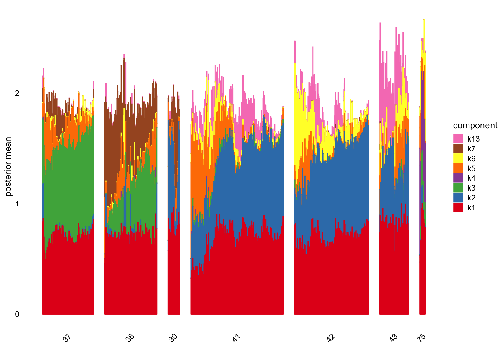

Version	Author	Date
7a353a3	junmingguan	2024-11-09


plot(flashier_fit_semi, 
     kset = which(ncells_semi > 5),
     plot_type = "structure",
     pm_which = "loadings", 
     pm_groups = data$cluster_id,
     bins = 30, gap = 70)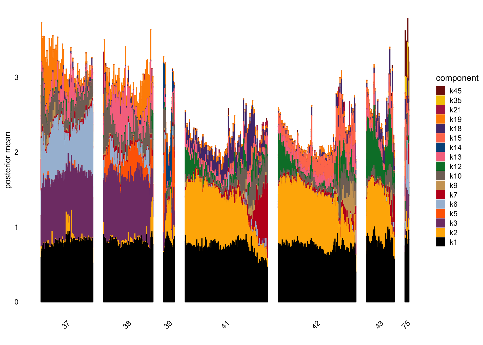

Version	Author	Date
7a353a3	junmingguan	2024-11-09

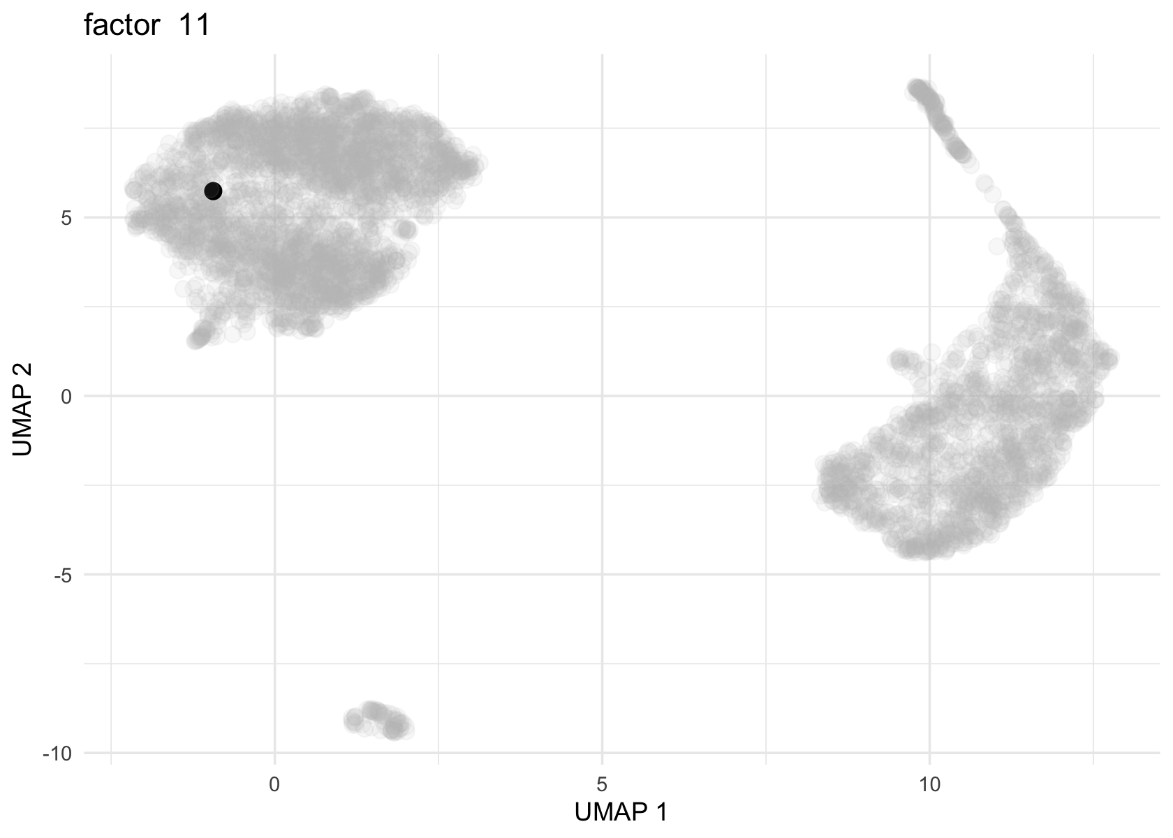
which.max(vals$L[, 8])
which.max(vals_semi$L[, 11])
# 10X390_3:GTTGTGAAGGCACGAT 
#                      1706 
# 10X390_3:GTTGTGAAGGCACGAT 
#                      1706

Both actor 8 from Flashier NMF and factor 11 from Flashier semi-NMF seem to be loaded on the same cell.

FastTopics

K = 50

plot_progress(fasttopics_fit_50,x = "iter",add.point.every = 10,colors = "black") +
  theme_cowplot(font_size = 10)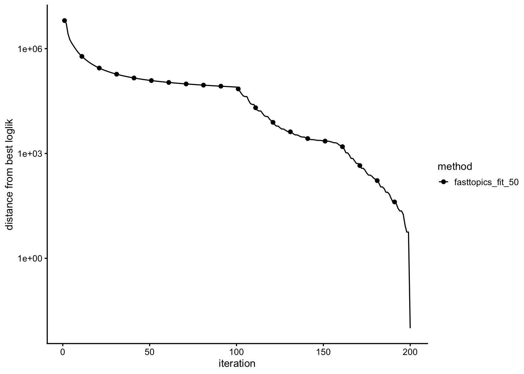

loglik <- loglik_multinom_topic_model(reduced_counts, fasttopics_fit_50)
pdat <- data.frame(loglik)
ggplot(pdat,aes(loglik)) +
  geom_histogram(bins = 64,color = "white",fill = "black",size = 0.25) +
  labs(y = "number of cells") +
  theme_cowplot(font_size = 10)
# Warning: Using `size` aesthetic for lines was deprecated in ggplot2 3.4.0.
# ℹ Please use `linewidth` instead.
# This warning is displayed once every 8 hours.
# Call `lifecycle::last_lifecycle_warnings()` to see where this warning was
# generated.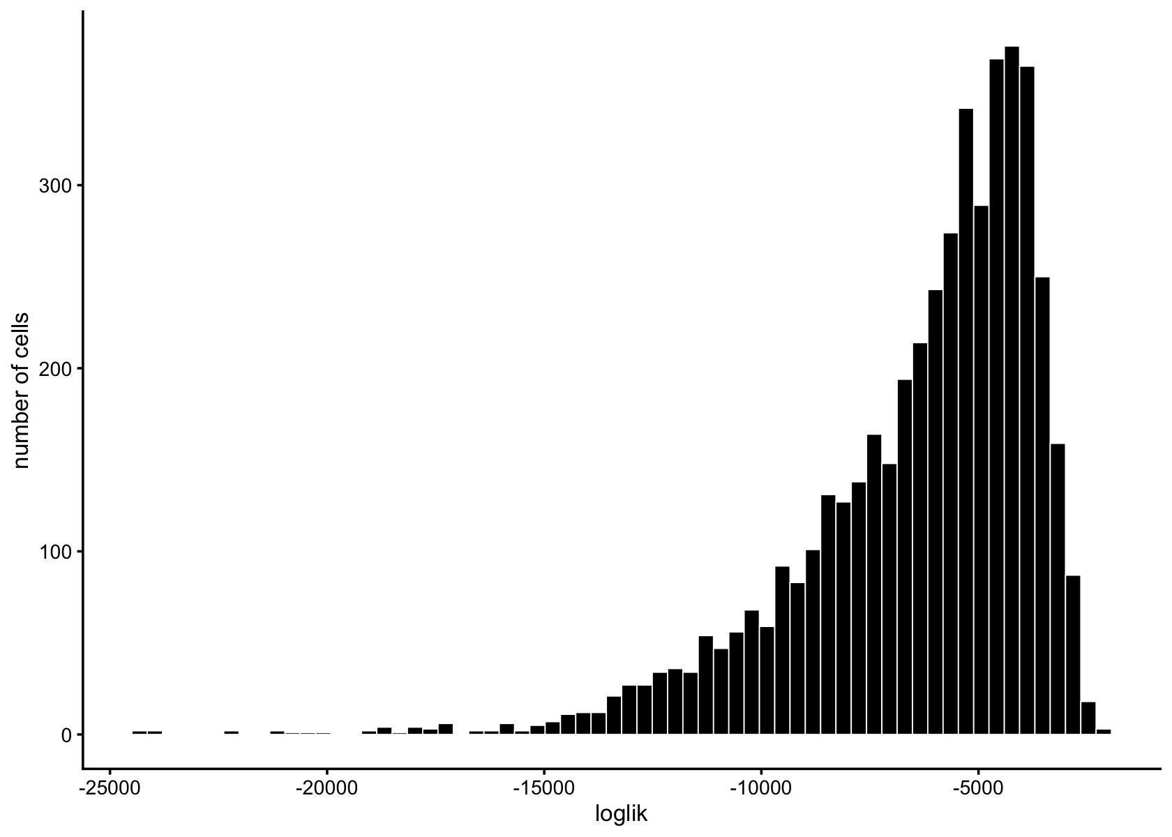


subpop_colors <- c("red", "blue", "green", "purple", "orange", "pink", "cyan", "brown", "yellow", "darkgreen")

pdat <- data.frame(loglik = loglik,subpop = data$cluster_id)
ggplot(pdat,aes(x = loglik,fill = subpop)) +
  geom_histogram(bins = 64,color = "white",size = 0.25) +
  scale_fill_manual(values = subpop_colors) +
  labs(y = "number of cells") +
  theme_cowplot(font_size = 10)

structure_plot(fasttopics_fit_50, grouping = data$cluster_id, gap = 70)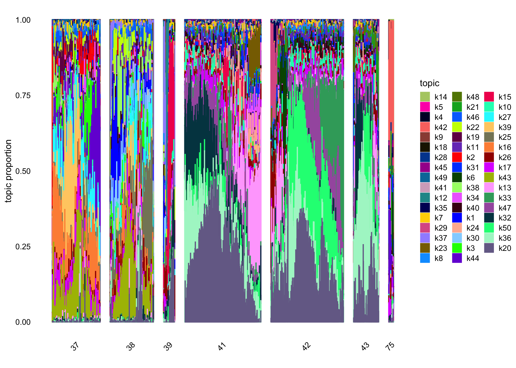

structure_plot(fasttopics_fit_50, grouping = subcluster_id, gap = 70)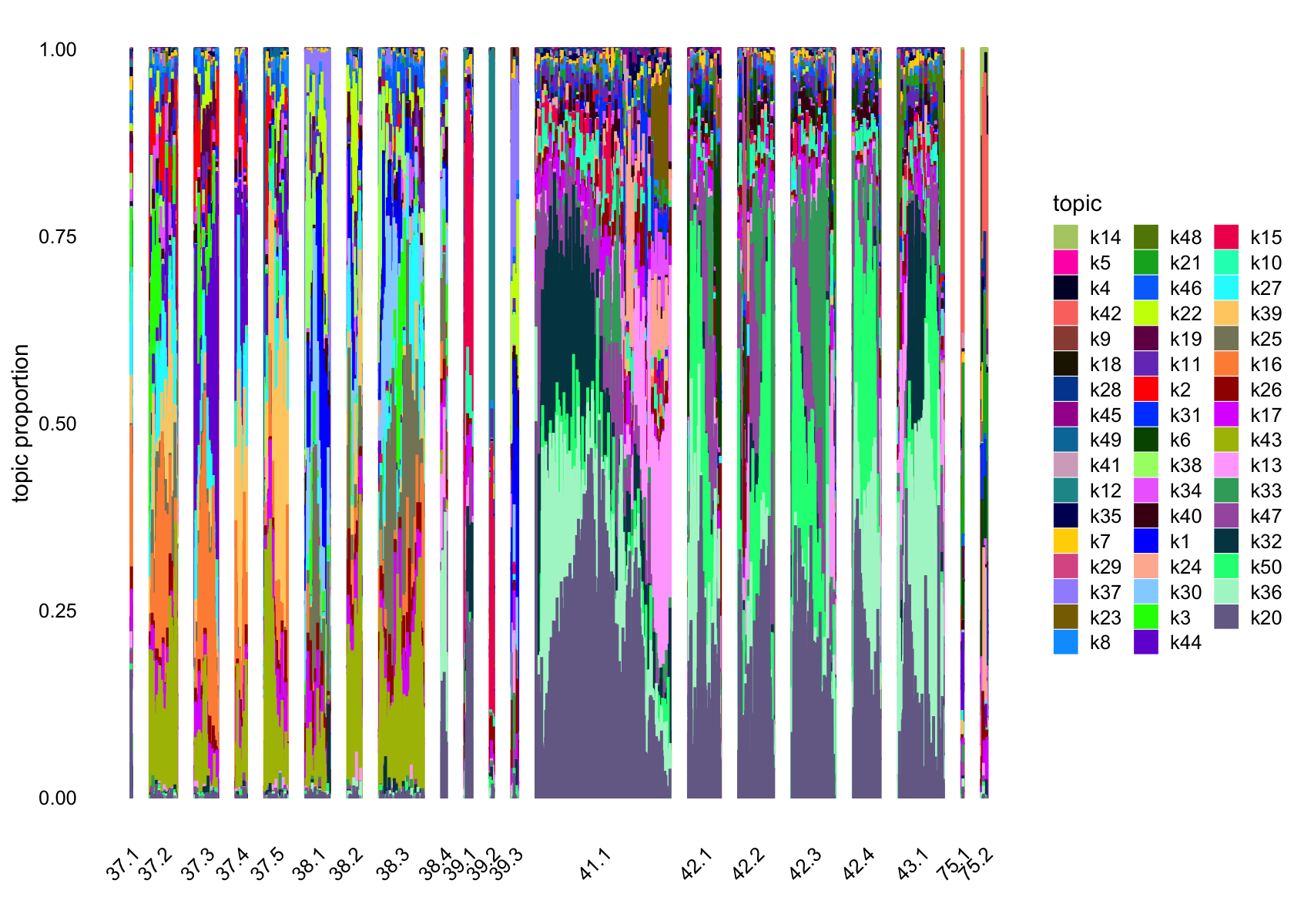

ncells_ft_50 <- colSums(fasttopics_fit_50$L>0.1)
ncells_ft_50
#   k1   k2   k3   k4   k5   k6   k7   k8   k9  k10  k11  k12  k13  k14  k15  k16 
#  251  252  355   22   25  138   10   10   51   49    7   70  552   46  217  449 
#  k17  k18  k19  k20  k21  k22  k23  k24  k25  k26  k27  k28  k29  k30  k31  k32 
#  113   70  205 1667  154  194  265  174  398  152  384   29  124  327  144  925 
#  k33  k34  k35  k36  k37  k38  k39  k40  k41  k42  k43  k44  k45  k46  k47  k48 
#  577  152   81 1025  163  267  354   13   75   61  518  297   45   92  889  136 
#  k49  k50 
#  101 1026

No factors that are loaded on a single cells. Still there are a couple that are loaded on a small number of cells, e.g., k11.

Removing factors that are loading on few than 200.

structure_plot(fasttopics_fit_50, topics = which(ncells_ft_50 >200),
               grouping = data$cluster_id, gap = 70)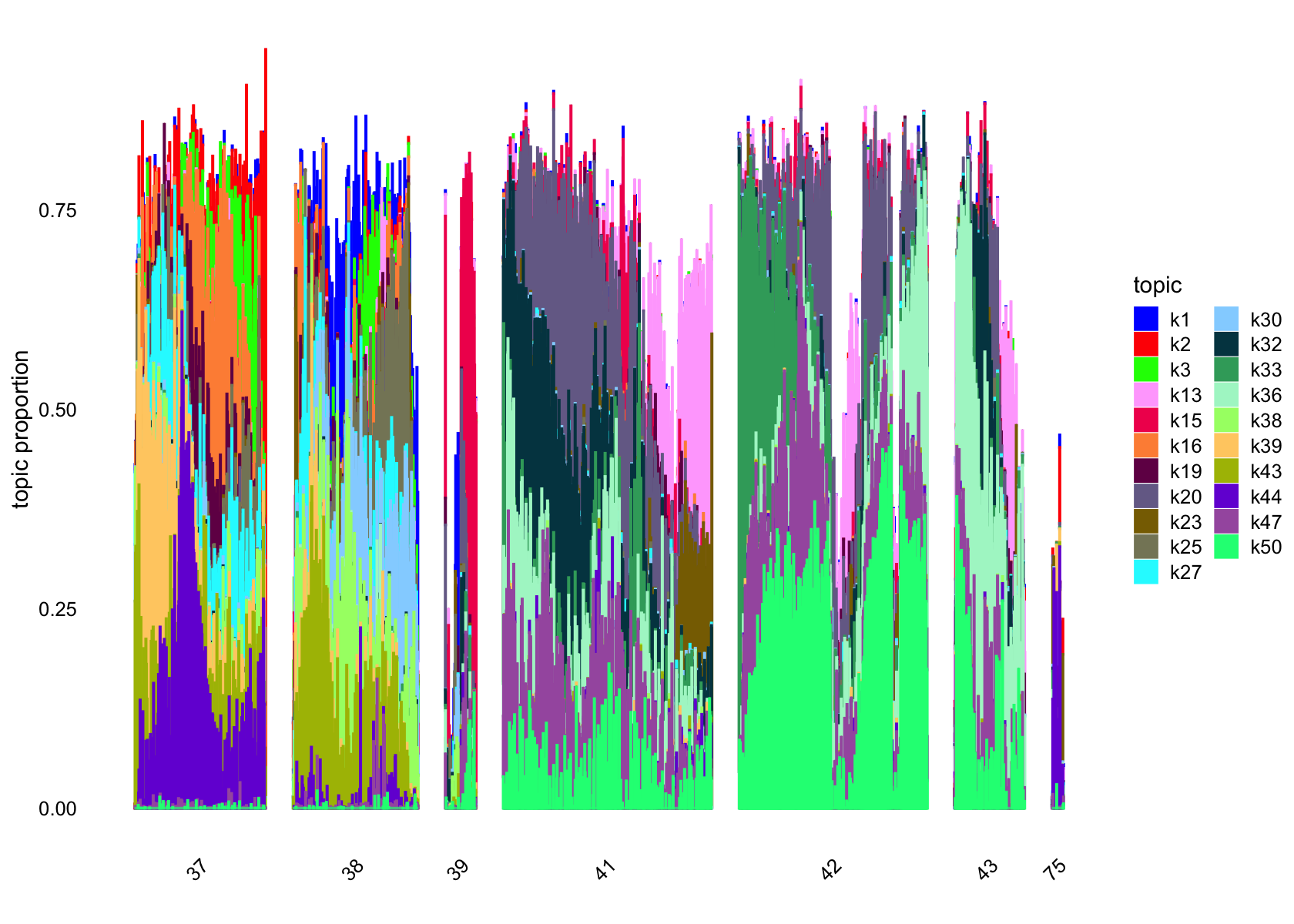

pca_plot(fasttopics_fit_50,fill = data$cluster_id)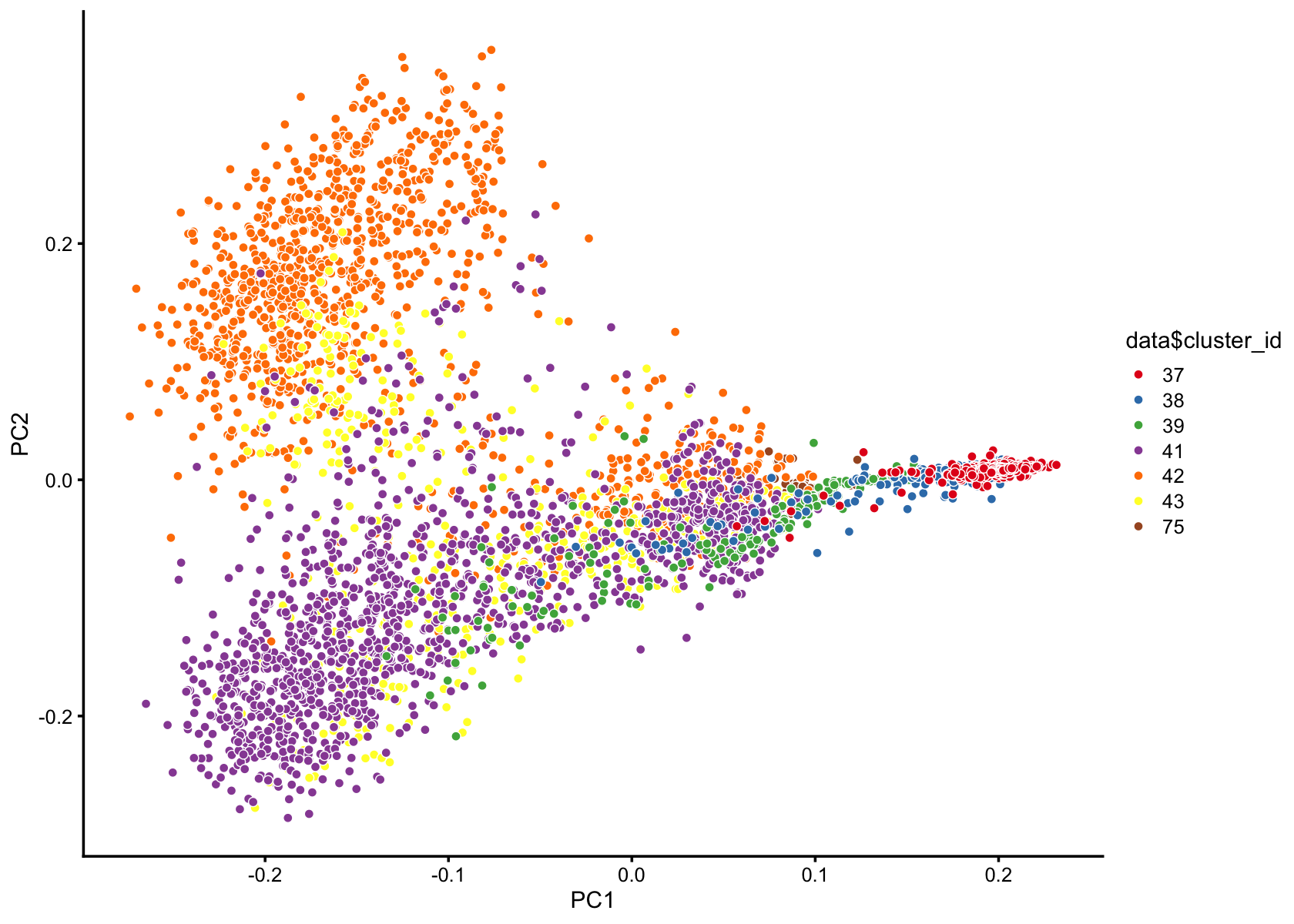

pca_hexbin_plot(fasttopics_fit_50,bins = 24)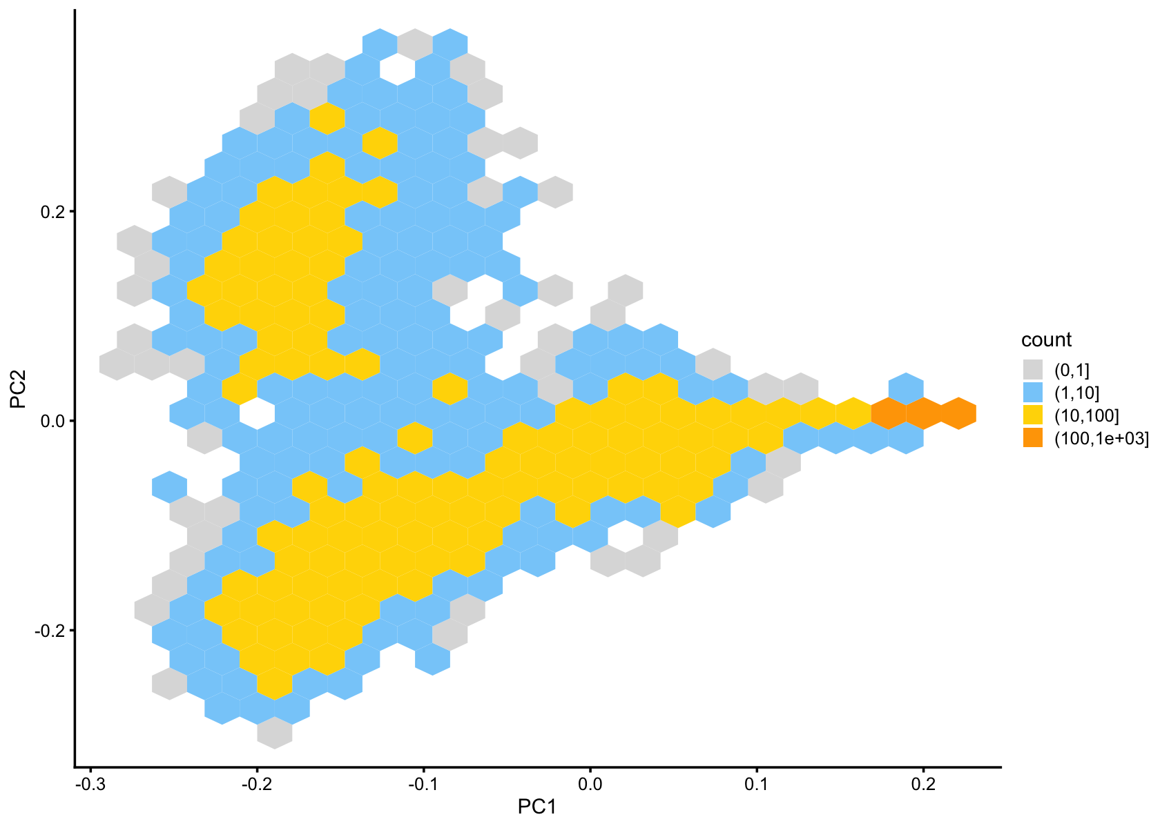

Top 5 driving genes for factors loaded on a few cells

top5_genes_factor_7 <- 
  sort(fasttopics_fit_50$F[, 7], decreasing = TRUE) %>% 
  head(., 5) %>%
  names()
homo_sapien_geno_info[match(top5_genes_factor_7, homo_sapien_geno_info$Ensembl),
                      c('Symbol', 'Ensembl')]
sort(fasttopics_fit_50$F[, 7], decreasing = TRUE) %>% 
  head(., 5)

top5_genes_factor_8 <- 
  sort(fasttopics_fit_50$F[, 8], decreasing = TRUE) %>% 
  head(., 5) %>%
  names()
homo_sapien_geno_info[match(top5_genes_factor_8, homo_sapien_geno_info$Ensembl),
                      c('Symbol', 'Ensembl')]
sort(fasttopics_fit_50$F[, 8], decreasing = TRUE) %>% 
  head(., 5)

top5_genes_factor_11 <- 
  sort(fasttopics_fit_50$F[, 11], decreasing = TRUE) %>% 
  head(., 5) %>%
  names()
homo_sapien_geno_info[match(top5_genes_factor_11, homo_sapien_geno_info$Ensembl),
                      c('Symbol', 'Ensembl')]

sort(fasttopics_fit_50$F[, 11], decreasing = TRUE) %>% 
  head(., 5)
#       Symbol         Ensembl
# 1661   ERBB4 ENSG00000178568
# 22566 MALAT1 ENSG00000251562
# 3257   LSAMP ENSG00000185565
# 20214  CADM2 ENSG00000175161
# 8975   NLGN1 ENSG00000169760
# ENSG00000178568 ENSG00000251562 ENSG00000185565 ENSG00000175161 ENSG00000169760 
#      0.11622755      0.03573029      0.02356664      0.01785754      0.01396652 
#        Symbol         Ensembl
# 4047    PDE4B ENSG00000184588
# 22566  MALAT1 ENSG00000251562
# 4357  PPP2R2B ENSG00000156475
# 20214   CADM2 ENSG00000175161
# 3257    LSAMP ENSG00000185565
# ENSG00000184588 ENSG00000251562 ENSG00000156475 ENSG00000175161 ENSG00000185565 
#      0.14022764      0.03307322      0.01717360      0.01491126      0.00890551 
#        Symbol         Ensembl
# 4357  PPP2R2B ENSG00000156475
# 15995   MAML2 ENSG00000184384
# 20214   CADM2 ENSG00000175161
# 21942  NCKAP5 ENSG00000176771
# 16290   FRMD5 ENSG00000171877
# ENSG00000156475 ENSG00000184384 ENSG00000175161 ENSG00000176771 ENSG00000171877 
#     0.262879278     0.005688911     0.005418745     0.004842882     0.004461895

ERBB4 (Receptor Tyrosine-Protein Kinase ErbB-4):
- Part of the EGFR family.
- Involved in cell growth, survival, and differentiation.
- Dysregulation is linked to cancer and neurodevelopmental disorders.
PDE4B (Phosphodiesterase 4B):
- Degrades cAMP, a secondary messenger in cellular signaling.
- Implicated in psychiatric conditions, including schizophrenia and depression.
PPP2R2B (Protein Phosphatase 2 Regulatory Subunit Bbeta):
- Regulates protein dephosphorylation.
- Associated with spinocerebellar ataxias and neurodegeneration. From chatgpt

K = 10

plot_progress(fasttopics_fit_10,x = "iter",add.point.every = 10,colors = "black") +
  theme_cowplot(font_size = 10)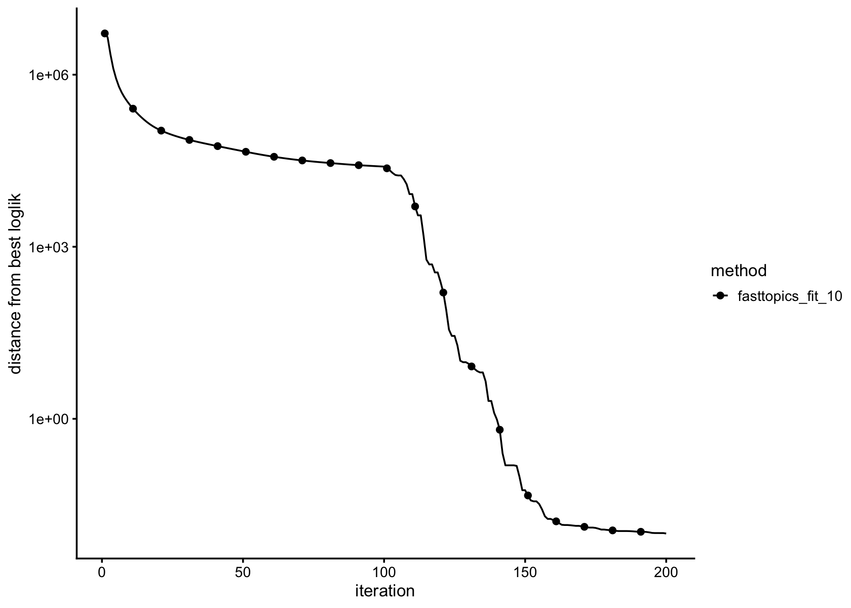

loglik <- loglik_multinom_topic_model(reduced_counts, fasttopics_fit_10)
pdat <- data.frame(loglik)
ggplot(pdat,aes(loglik)) +
  geom_histogram(bins = 64,color = "white",fill = "black",size = 0.25) +
  labs(y = "number of cells") +
  theme_cowplot(font_size = 10)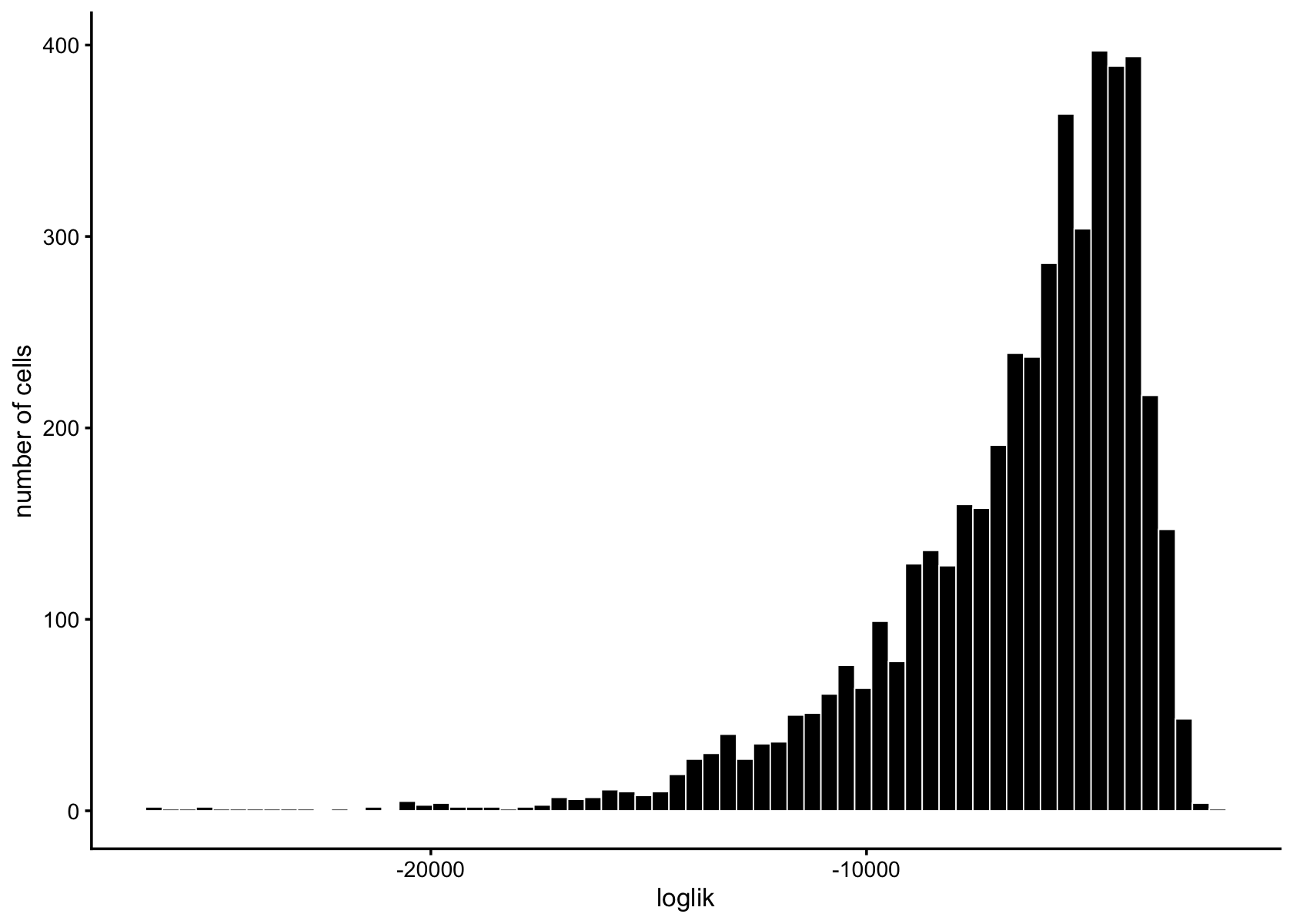


subpop_colors <- c("red", "blue", "green", "purple", "orange", "pink", "cyan", "brown", "yellow", "darkgreen")

pdat <- data.frame(loglik = loglik,subpop = data$cluster_id)
ggplot(pdat,aes(x = loglik,fill = subpop)) +
  geom_histogram(bins = 64,color = "white",size = 0.25) +
  scale_fill_manual(values = subpop_colors) +
  labs(y = "number of cells") +
  theme_cowplot(font_size = 10)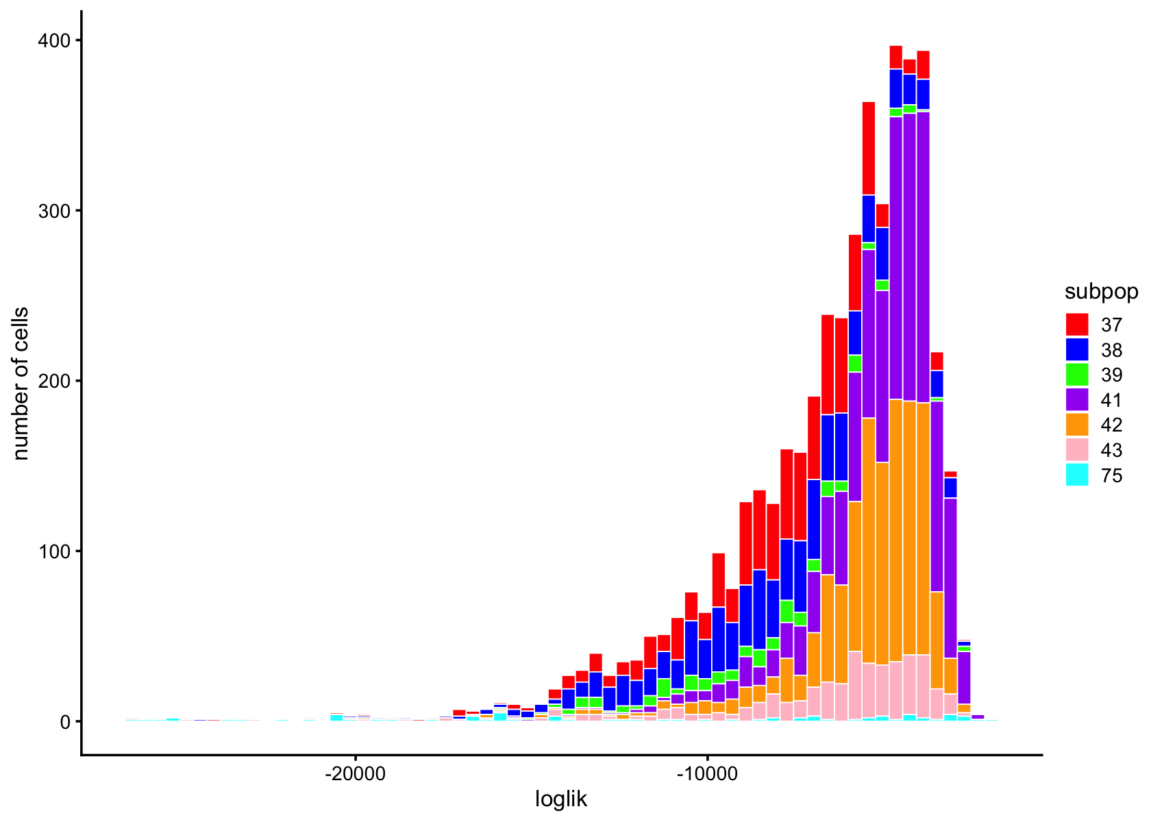

structure_plot(fasttopics_fit_10, grouping = data$cluster_id, gap = 70)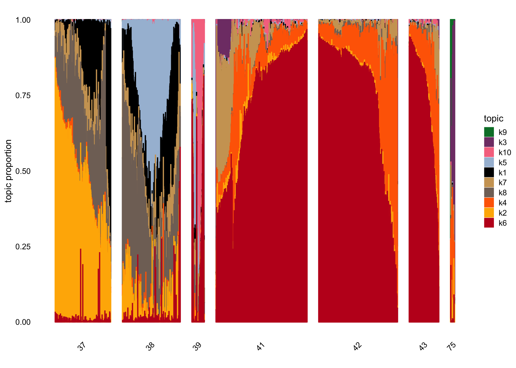

structure_plot(fasttopics_fit_10, grouping = subcluster_id, gap = 70)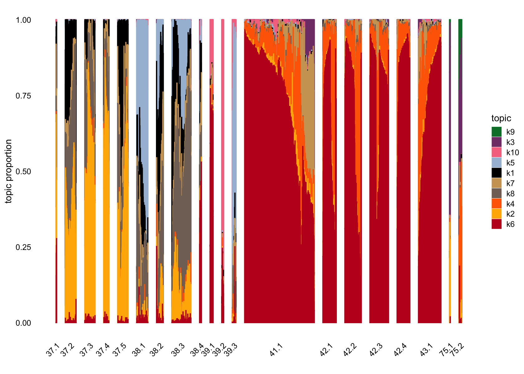

ncells_ft_10 <- colSums(fasttopics_fit_10$L>0.1)
ncells_ft_10
#   k1   k2   k3   k4   k5   k6   k7   k8   k9  k10 
# 1140  976  394 1141  671 3011 1360 1276   61  234

Removing factor 9

structure_plot(fasttopics_fit_10, topics = which(ncells_ft_10 > 61),
               grouping = data$cluster_id, gap = 70)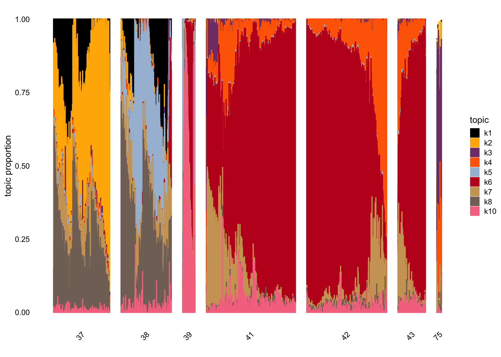

structure_plot(fasttopics_fit_10, topics = which(ncells_ft_10 > 61),
               grouping = subcluster_id, gap = 70)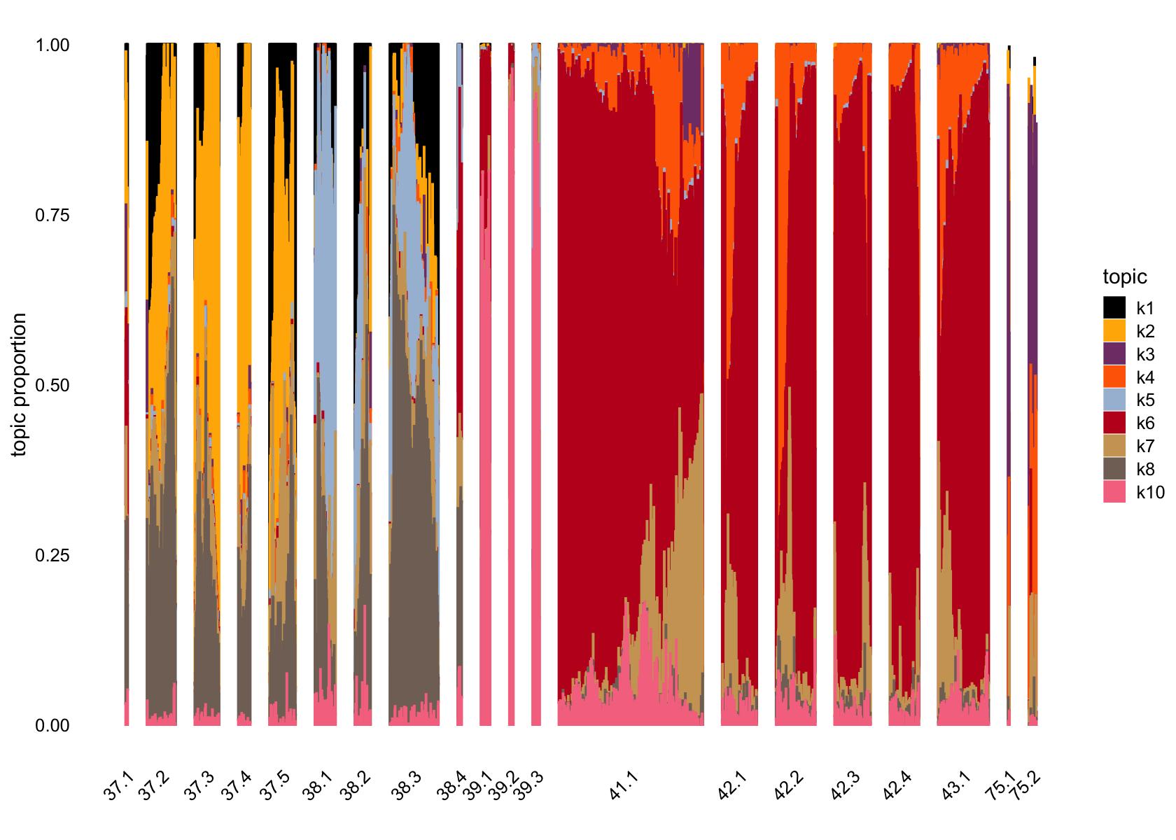

pca_plot(fasttopics_fit_10,fill = data$cluster_id)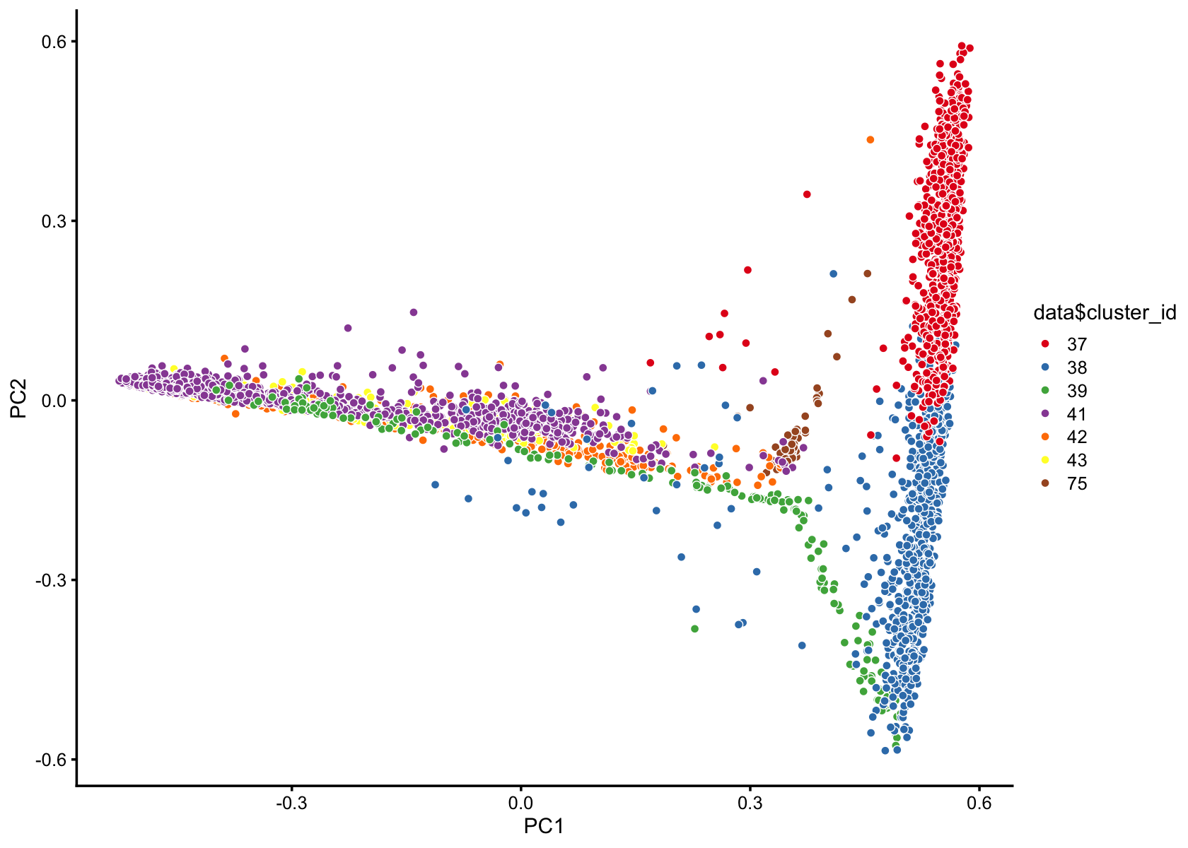

pca_hexbin_plot(fasttopics_fit_10,bins = 24)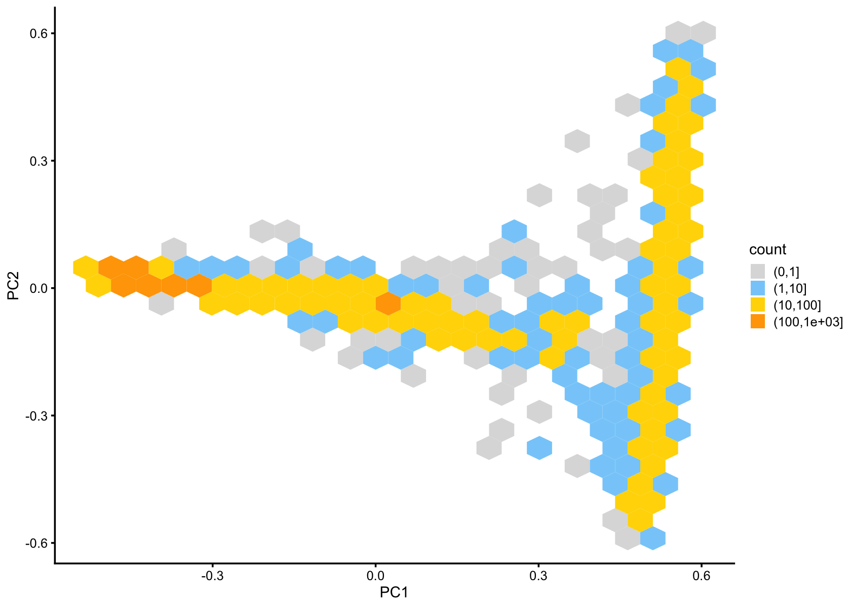

top5_genes_factor_9 <- 
  sort(fasttopics_fit_10$F[, 9], decreasing = TRUE) %>% 
  head(., 5) %>%
  names()
homo_sapien_geno_info[match(top5_genes_factor_9, homo_sapien_geno_info$Ensembl),
                      c('Symbol', 'Ensembl')]
sort(fasttopics_fit_10$F[, 9], decreasing = TRUE) %>% 
  head(., 5)
#       Symbol         Ensembl
# 5839     TTR ENSG00000118271
# 22566 MALAT1 ENSG00000251562
# 15061  TRPM3 ENSG00000083067
# 2734   HTR2C ENSG00000147246
# 15202 KCNIP4 ENSG00000185774
# ENSG00000118271 ENSG00000251562 ENSG00000083067 ENSG00000147246 ENSG00000185774 
#     0.191939663     0.023044075     0.005731441     0.003988197     0.003979024

“TTR encodes Transthyretin, a protein primarily synthesized in the liver and choroid plexus of the brain.” From chatGPT

GBCD

TODO

# source("../code/fit_cov_ebnmf.R")
# 
# fit.gbcd <-
#   flash_fit_cov_ebnmf(Y = reduced_counts, Kmax = 7,
#                       prior = flash_ebnm(prior_family = "generalized_binary",
#                                          scale = 0.04),
#                       extrapolate = FALSE)

sessionInfo()
# R version 4.3.1 (2023-06-16)
# Platform: aarch64-apple-darwin20 (64-bit)
# Running under: macOS Sonoma 14.5
# 
# Matrix products: default
# BLAS:   /Library/Frameworks/R.framework/Versions/4.3-arm64/Resources/lib/libRblas.0.dylib 
# LAPACK: /Library/Frameworks/R.framework/Versions/4.3-arm64/Resources/lib/libRlapack.dylib;  LAPACK version 3.11.0
# 
# locale:
# [1] en_US.UTF-8/en_US.UTF-8/en_US.UTF-8/C/en_US.UTF-8/en_US.UTF-8
# 
# time zone: America/Chicago
# tzcode source: internal
# 
# attached base packages:
# [1] stats     graphics  grDevices utils     datasets  methods   base     
# 
# other attached packages:
#  [1] SeuratObject_5.0.2 sp_2.1-4           knitr_1.48         readr_2.1.4       
#  [5] dplyr_1.1.4        cowplot_1.1.3      ggplot2_3.5.1      fastTopics_0.6-192
#  [9] flashier_1.0.54    ebnm_1.1-34        Matrix_1.6-4      
# 
# loaded via a namespace (and not attached):
#  [1] pbapply_1.7-2        rlang_1.1.4          magrittr_2.0.3      
#  [4] git2r_0.35.0         horseshoe_0.2.0      compiler_4.3.1      
#  [7] vctrs_0.6.5          quadprog_1.5-8       stringr_1.5.1       
# [10] pkgconfig_2.0.3      crayon_1.5.3         fastmap_1.2.0       
# [13] labeling_0.4.3       utf8_1.2.4           promises_1.3.0      
# [16] rmarkdown_2.28       tzdb_0.4.0           purrr_1.0.2         
# [19] bit_4.0.5            xfun_0.48            cachem_1.1.0        
# [22] trust_0.1-8          jsonlite_1.8.9       progress_1.2.3      
# [25] highr_0.11           later_1.3.2          irlba_2.3.5.1       
# [28] parallel_4.3.1       prettyunits_1.2.0    R6_2.5.1            
# [31] bslib_0.8.0          stringi_1.8.4        RColorBrewer_1.1-3  
# [34] SQUAREM_2021.1       parallelly_1.38.0    jquerylib_0.1.4     
# [37] Rcpp_1.0.13          future.apply_1.11.3  httpuv_1.6.14       
# [40] splines_4.3.1        tidyselect_1.2.1     rstudioapi_0.15.0   
# [43] yaml_2.3.10          codetools_0.2-19     listenv_0.9.1       
# [46] lattice_0.21-8       tibble_3.2.1         withr_3.0.2         
# [49] evaluate_1.0.1       Rtsne_0.17           future_1.34.0       
# [52] RcppParallel_5.1.9   pillar_1.9.0         whisker_0.4.1       
# [55] plotly_4.10.4        softImpute_1.4-1     generics_0.1.3      
# [58] vroom_1.6.3          rprojroot_2.0.3      invgamma_1.1        
# [61] truncnorm_1.0-9      hms_1.1.3            munsell_0.5.1       
# [64] scales_1.3.0         ashr_2.2-63          gtools_3.9.5        
# [67] globals_0.16.3       RhpcBLASctl_0.23-42  glue_1.8.0          
# [70] scatterplot3d_0.3-44 lazyeval_0.2.2       tools_4.3.1         
# [73] hexbin_1.28.5        data.table_1.16.2    dotCall64_1.2       
# [76] fs_1.6.4             grid_4.3.1           tidyr_1.3.1         
# [79] colorspace_2.1-1     deconvolveR_1.2-1    cli_3.6.3           
# [82] Polychrome_1.5.1     workflowr_1.7.1      spam_2.11-0         
# [85] fansi_1.0.6          mixsqp_0.3-54        viridisLite_0.4.2   
# [88] uwot_0.1.16          gtable_0.3.6         sass_0.4.9          
# [91] digest_0.6.37        progressr_0.14.0     ggrepel_0.9.6       
# [94] farver_2.1.2         htmlwidgets_1.6.4    htmltools_0.5.8.1   
# [97] lifecycle_1.0.4      httr_1.4.7           bit64_4.0.5

Initial exploration of the human brain dataset: committed OPC cells

Junming Guan

Introduction

t-SNE and UMAP

t-SNE

UMAP

Flashier

NMF

Loadings on UMAP by factor

Semi-NMF

Loadings on UMAP by factor

Comparison

FastTopics

K = 50

K = 10

GBCD