NMF analysis of the combined tissue + organoid GCA data
Peter Carbonetto
Last updated: 2026-04-13
Checks: 7 0
Knit directory:
single-cell-jamboree/analysis/
This reproducible R Markdown analysis was created with workflowr (version 1.7.1). The Checks tab describes the reproducibility checks that were applied when the results were created. The Past versions tab lists the development history.
Great! Since the R Markdown file has been committed to the Git repository, you know the exact version of the code that produced these results.
Great job! The global environment was empty. Objects defined in the global environment can affect the analysis in your R Markdown file in unknown ways. For reproduciblity it’s best to always run the code in an empty environment.
The command set.seed(1) was run prior to running the
code in the R Markdown file. Setting a seed ensures that any results
that rely on randomness, e.g. subsampling or permutations, are
reproducible.
Great job! Recording the operating system, R version, and package versions is critical for reproducibility.
Nice! There were no cached chunks for this analysis, so you can be confident that you successfully produced the results during this run.
Great job! Using relative paths to the files within your workflowr project makes it easier to run your code on other machines.
Great! You are using Git for version control. Tracking code development and connecting the code version to the results is critical for reproducibility.
The results in this page were generated with repository version 20607df. See the Past versions tab to see a history of the changes made to the R Markdown and HTML files.
Note that you need to be careful to ensure that all relevant files for
the analysis have been committed to Git prior to generating the results
(you can use wflow_publish or
wflow_git_commit). workflowr only checks the R Markdown
file, but you know if there are other scripts or data files that it
depends on. Below is the status of the Git repository when the results
were generated:
Untracked files:
    Untracked:  analysis/lps_cache/
    Untracked:  analysis/mcf7_cache/
    Untracked:  data/GSE125162_ALL-fastqTomat0-Counts.tsv.gz
    Untracked:  data/GSE128565/
    Untracked:  data/GSE132188_adata.h5ad.h5
    Untracked:  data/GSE156175_RAW/
    Untracked:  data/GSE183010/
    Untracked:  data/Immune_ALL_human.h5ad
    Untracked:  data/pancreas_cytokine.RData
    Untracked:  data/pancreas_cytokine_lsa.RData
    Untracked:  data/pancreas_cytokine_lsa_v2.RData
    Untracked:  data/pancreas_endocrine.RData
    Untracked:  data/pancreas_endocrine_alldays.h5ad
    Untracked:  data/yeast.RData

Unstaged changes:
    Modified:   analysis/gca.R
    Modified:   analysis/lps.Rmd
Note that any generated files, e.g. HTML, png, CSS, etc., are not included in this status report because it is ok for generated content to have uncommitted changes.
These are the previous versions of the repository in which changes were
made to the R Markdown (analysis/gca.Rmd) and HTML
(docs/gca.html) files. If you’ve configured a remote Git
repository (see ?wflow_git_remote), click on the hyperlinks
in the table below to view the files as they were in that past version.
| File | Version | Author | Date | Message |
|---|---|---|---|---|
| Rmd | 20607df | Peter Carbonetto | 2026-04-13 | wflow_publish("gca.Rmd", verbose = T, view = F) |
| html | cf4bf67 | Peter Carbonetto | 2026-03-17 | Improved the coloring of the structure plots in the gca analysis. |
| Rmd | 7e5b3fd | Peter Carbonetto | 2026-03-17 | wflow_publish("gca.Rmd", verbose = T, view = F) |
| html | 0284003 | Peter Carbonetto | 2026-03-17 | Subsampled the EC cells for the structure plots in the gca analysis. |
| Rmd | 4a1993a | Peter Carbonetto | 2026-03-17 | wflow_publish("gca.Rmd", verbose = T, view = F) |
| html | 96c0613 | Peter Carbonetto | 2026-03-16 | Ran wflow_publish("gca.Rmd"). |
| Rmd | f6d72d2 | Peter Carbonetto | 2026-03-16 | wflow_publish("gca.Rmd", verbose = T, view = F) |
| Rmd | 82c9fdb | Peter Carbonetto | 2026-03-16 | Made some adjustments to the structure plots in gca.Rmd. |
| Rmd | dc2cdfb | Peter Carbonetto | 2026-03-16 | Working on structure plots in gca analysis. |
| Rmd | 94b4614 | Peter Carbonetto | 2026-03-16 | Working on the structure plots in gca.Rmd. |
| html | f1fbc12 | Peter Carbonetto | 2026-03-16 | First build of the gca analysis. |
| Rmd | 73025b1 | Peter Carbonetto | 2026-03-16 | wflow_publish("gca.Rmd", view = F, verbose = T) |
Here we explore whether non-negative matrix factorization (NMF)
identifies factors (i.e., gene programs) common to both the tissues and
organoids. These results were generated using the
fit_gca_nmf.R script, found here.
Load the packages needed for this analysis:
library(ggplot2)
library(cowplot)
library(fastTopics)
Set the seed for reproducibility:
set.seed(1)Load the results from running fitting an NMF model using flashier, with \(k = 30\):
load("../output/gca_nmf_k=20.RData")
L <- fl_nmf_ldf$L
colnames(L) <- paste0("k",1:20)
For better Structure Plots, subsample the EC cells:
rows1 <- which(sample_info$celltype == "EC")
rows2 <- which(sample_info$celltype != "EC")
rows1 <- sample(rows1,8000)
rows  <- c(rows1,rows2)
rows  <- sort(rows)
L     <- L[rows,]
sample_info <- sample_info[rows,]
These are the factors (gene programs) that are mostly specific to tissues. Observe that the memberships in the organoids (bottom) are mostly very small.
topics_tissue <- c("k2","k3","k9","k12","k14","k15","k20")
topic_colors <-
  c("#FFB300","#803E75","#FF6800","#A6BDD7","#C10020","#CEA262",
    "#93AA00","#007D34","#F6768E","#00538A","#FF7A5C","darkblue",
    "#FF8E00","yellow","cyan","#F4C800","#817066","#593315",
    "#F13A13","forestgreen")
rows1 <- which(sample_info$origin == "Tissue")
rows2 <- which(sample_info$origin == "Org")
p1 <- structure_plot(L[rows1,],gap = 10,topics = topics_tissue,
                     grouping = factor(sample_info[rows1,"celltype"]),
                     colors = topic_colors) +
  labs(y = "membership",title = "tissues")
p2 <- structure_plot(L[rows2,],gap = 10,topics = topics_tissue,
                     grouping = factor(sample_info[rows2,"celltype"]),
                     colors = topic_colors) +
  labs(y = "membership",title = "organoids") +
  ylim(0,1)
plot_grid(p1,p2,nrow = 2,ncol = 1)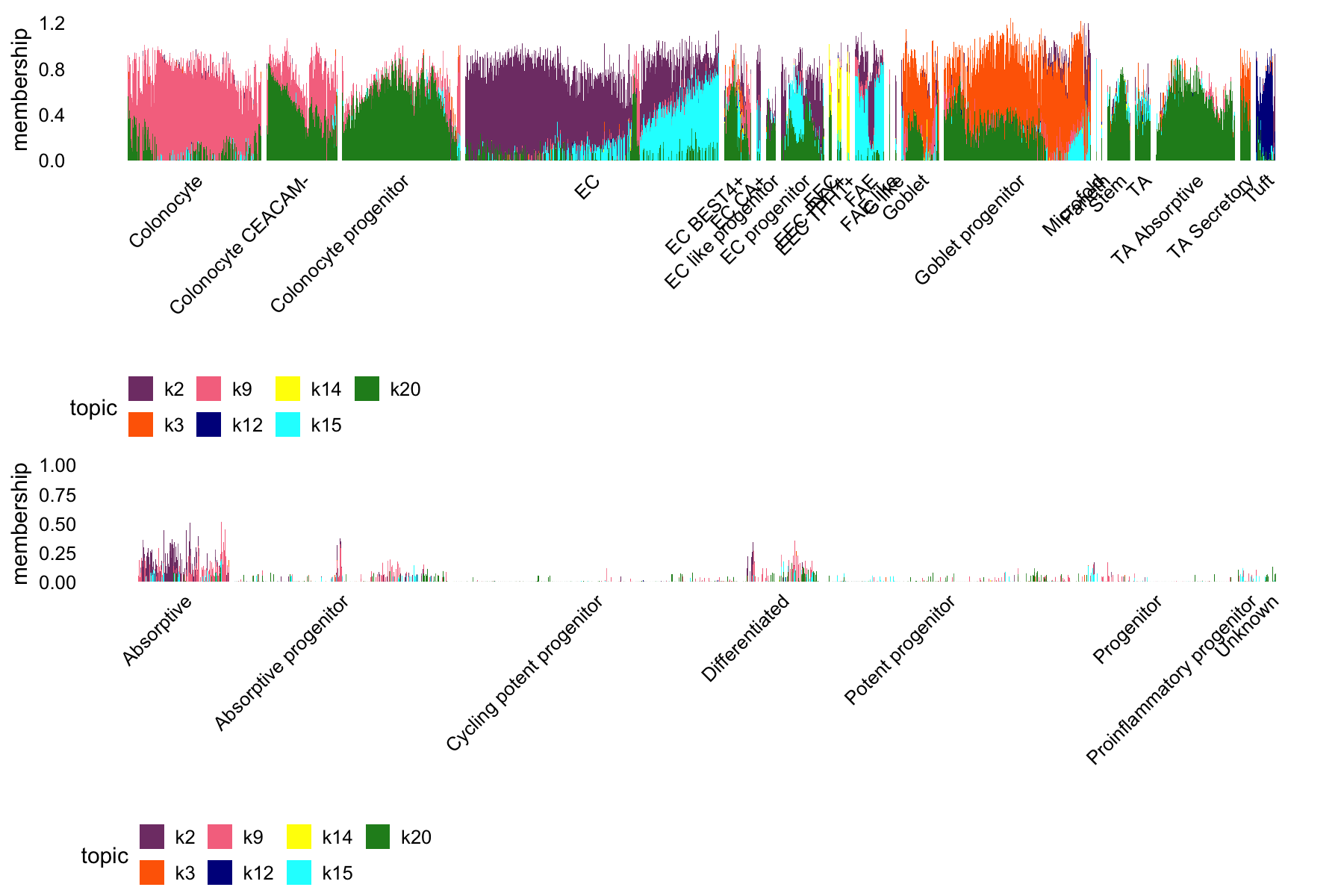
Note: that I’m using the cell-type labels in the “celltype” column of the meta data as a reference point for understanding the gene programs.
Next, these are the gene programs mostly specific to organoids. Again, notice that the memberships are mostly very small in the tissues:
topics_organoid <- c("k4","k6","k8","k11","k13","k17","k18")
rows1 <- which(sample_info$origin == "Tissue")
rows2 <- which(sample_info$origin == "Org")
p3 <- structure_plot(L[rows1,],gap = 10,topics = topics_organoid,
                     grouping = factor(sample_info[rows1,"celltype"]),
                     colors = topic_colors) +
  labs(y = "membership",title = "tissues") +
  ylim(0,2)
p4 <- structure_plot(L[rows2,],gap = 10,topics = topics_organoid,
                     grouping = factor(sample_info[rows2,"celltype"]),
                     colors = topic_colors) +
  labs(y = "membership",title = "organoids")
plot_grid(p3,p4,nrow = 2,ncol = 1)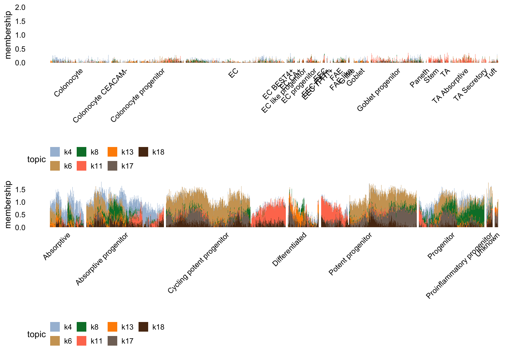
Finally, these are the gene programs that appear in both the tissues and the organoids.
topics_shared <- c("k5","k7","k10","k16","k19")
rows1 <- which(sample_info$origin == "Tissue")
rows2 <- which(sample_info$origin == "Org")
p5 <- structure_plot(L[rows1,],gap = 10,topics = topics_shared,
                     grouping = factor(sample_info[rows1,"celltype"]),
                     colors = topic_colors) +
  labs(y = "membership",title = "tissues")
p6 <- structure_plot(L[rows2,],gap = 10,topics = topics_shared,
                     grouping = factor(sample_info[rows2,"celltype"]),
                     colors = topic_colors) +
  labs(y = "membership",title = "organoids")
plot_grid(p5,p6,nrow = 2,ncol = 1)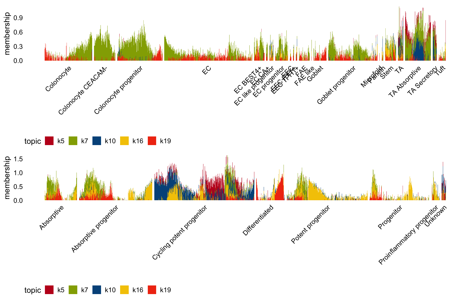
In organoids, factor 16 is most active in the TI, in non-CD-adj groups:
rows1 <- with(sample_info,
              which(region == "TI" & group != "CD adj" & origin == "Org"))
rows2 <- with(sample_info,
              which(!(region == "TI" & group != "CD adj") & origin == "Org"))
p7 <- structure_plot(L[rows1,],gap = 10,topics = topics_shared,
                     grouping = factor(sample_info[rows1,"celltype"]),
                     colors = topic_colors) +
  labs(y = "membership",title = "TI, non-CD-adj")
p8 <- structure_plot(L[rows2,],gap = 10,topics = topics_shared,
                     grouping = factor(sample_info[rows2,"celltype"]),
                     colors = topic_colors) +
  labs(y = "membership",title = "all other cells")
plot_grid(p7,p8,nrow = 2,ncol = 1)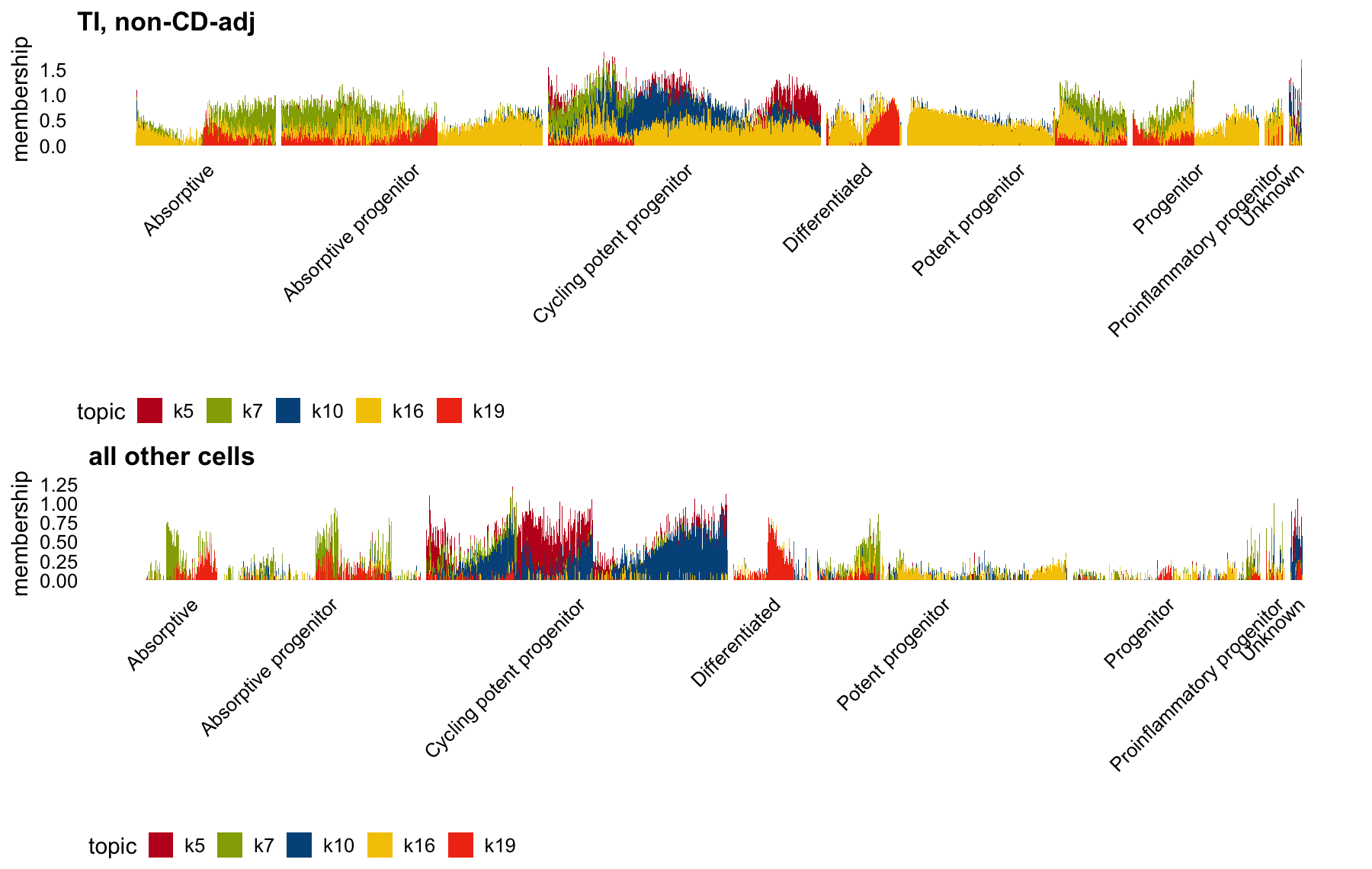
In organoids, factor 7 is most active in the non-CD-adj cells:
rows1 <- with(sample_info,which(group != "CD adj" & origin == "Org"))
rows2 <- with(sample_info,which(group == "CD adj" & origin == "Org"))
p9 <- structure_plot(L[rows1,],gap = 10,topics = topics_shared,
                     grouping = factor(sample_info[rows1,"celltype"]),
                     colors = topic_colors) +
  labs(y = "membership",title = "organoids (non-CD-adj)")
p10 <- structure_plot(L[rows2,],gap = 10,topics = topics_shared,
                      grouping = factor(sample_info[rows2,"celltype"]),
                      colors = topic_colors) +
  labs(y = "membership",title = "organoids (CD-adj)")
plot_grid(p9,p10,nrow = 2,ncol = 1)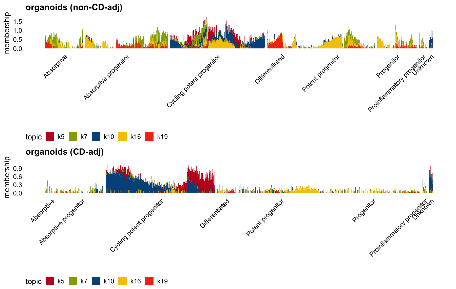
sessionInfo()
# R version 4.3.3 (2024-02-29)
# Platform: aarch64-apple-darwin20 (64-bit)
# Running under: macOS 15.7.4
#
# Matrix products: default
# BLAS:   /System/Library/Frameworks/Accelerate.framework/Versions/A/Frameworks/vecLib.framework/Versions/A/libBLAS.dylib
# LAPACK: /Library/Frameworks/R.framework/Versions/4.3-arm64/Resources/lib/libRlapack.dylib;  LAPACK version 3.11.0
#
# locale:
# [1] en_US.UTF-8/en_US.UTF-8/en_US.UTF-8/C/en_US.UTF-8/en_US.UTF-8
#
# time zone: America/Chicago
# tzcode source: internal
#
# attached base packages:
# [1] stats     graphics  grDevices utils     datasets  methods   base
#
# other attached packages:
# [1] fastTopics_0.7-38 cowplot_1.1.3     ggplot2_3.5.2
#
# loaded via a namespace (and not attached):
#  [1] gtable_0.3.6        xfun_0.52           bslib_0.9.0
#  [4] htmlwidgets_1.6.4   ggrepel_0.9.6       lattice_0.22-5
#  [7] quadprog_1.5-8      vctrs_0.6.5         tools_4.3.3
# [10] generics_0.1.4      parallel_4.3.3      tibble_3.3.0
# [13] pkgconfig_2.0.3     Matrix_1.6-5        data.table_1.17.6
# [16] SQUAREM_2021.1      RColorBrewer_1.1-3  RcppParallel_5.1.10
# [19] lifecycle_1.0.4     truncnorm_1.0-9     compiler_4.3.3
# [22] farver_2.1.2        stringr_1.5.1       git2r_0.33.0
# [25] progress_1.2.3      RhpcBLASctl_0.23-42 httpuv_1.6.14
# [28] htmltools_0.5.8.1   sass_0.4.10         yaml_2.3.10
# [31] lazyeval_0.2.2      plotly_4.11.0       later_1.4.2
# [34] pillar_1.11.0       crayon_1.5.3        jquerylib_0.1.4
# [37] whisker_0.4.1       tidyr_1.3.1         uwot_0.2.3
# [40] cachem_1.1.0        gtools_3.9.5        tidyselect_1.2.1
# [43] digest_0.6.37       Rtsne_0.17          stringi_1.8.7
# [46] reshape2_1.4.4      dplyr_1.1.4         purrr_1.0.4
# [49] ashr_2.2-66         labeling_0.4.3      rprojroot_2.0.4
# [52] fastmap_1.2.0       grid_4.3.3          cli_3.6.5
# [55] invgamma_1.2        magrittr_2.0.3      dichromat_2.0-0.1
# [58] withr_3.0.2         prettyunits_1.2.0   scales_1.4.0
# [61] promises_1.3.3      rmarkdown_2.29      httr_1.4.7
# [64] workflowr_1.7.1     hms_1.1.3           pbapply_1.7-2
# [67] evaluate_1.0.4      knitr_1.50          irlba_2.3.5.1
# [70] viridisLite_0.4.2   rlang_1.1.6         Rcpp_1.1.0
# [73] mixsqp_0.3-54       glue_1.8.0          jsonlite_2.0.0
# [76] plyr_1.8.9          R6_2.6.1            fs_1.6.6