Initial exploration of the budding yeast data set
Peter Carbonetto
Last updated: 2025-08-13
Checks: 7 0
Knit directory:
single-cell-jamboree/analysis/
This reproducible R Markdown analysis was created with workflowr (version 1.7.1). The Checks tab describes the reproducibility checks that were applied when the results were created. The Past versions tab lists the development history.
Great! Since the R Markdown file has been committed to the Git repository, you know the exact version of the code that produced these results.
Great job! The global environment was empty. Objects defined in the global environment can affect the analysis in your R Markdown file in unknown ways. For reproduciblity it’s best to always run the code in an empty environment.
The command set.seed(1) was run prior to running the
code in the R Markdown file. Setting a seed ensures that any results
that rely on randomness, e.g. subsampling or permutations, are
reproducible.
Great job! Recording the operating system, R version, and package versions is critical for reproducibility.
Nice! There were no cached chunks for this analysis, so you can be confident that you successfully produced the results during this run.
Great job! Using relative paths to the files within your workflowr project makes it easier to run your code on other machines.
Great! You are using Git for version control. Tracking code development and connecting the code version to the results is critical for reproducibility.
The results in this page were generated with repository version b99041c. See the Past versions tab to see a history of the changes made to the R Markdown and HTML files.
Note that you need to be careful to ensure that all relevant files for
the analysis have been committed to Git prior to generating the results
(you can use wflow_publish or
wflow_git_commit). workflowr only checks the R Markdown
file, but you know if there are other scripts or data files that it
depends on. Below is the status of the Git repository when the results
were generated:
Untracked files:
    Untracked:  analysis/lps_cache/
    Untracked:  analysis/lps_fl_nmf_k6.csv
    Untracked:  analysis/lps_gsea_fl_nmf_k6.csv
    Untracked:  analysis/mcf7_cache/
    Untracked:  analysis/pancreas_cytokine_S1_factors_cache/
    Untracked:  analysis/pancreas_cytokine_lsa_clustering_cache/
    Untracked:  analysis/yeast.RData
    Untracked:  data/GSE125162_ALL-fastqTomat0-Counts.tsv.gz
    Untracked:  data/GSE132188_adata.h5ad.h5
    Untracked:  data/GSE156175_RAW/
    Untracked:  data/GSE183010/
    Untracked:  data/Immune_ALL_human.h5ad
    Untracked:  data/pancreas_cytokine.RData
    Untracked:  data/pancreas_cytokine_lsa.RData
    Untracked:  data/pancreas_cytokine_lsa_v2.RData
    Untracked:  data/pancreas_endocrine.RData
    Untracked:  data/pancreas_endocrine_alldays.h5ad
    Untracked:  output/panc_cyto_lsa_res/

Unstaged changes:
    Modified:   analysis/lps.Rmd
Note that any generated files, e.g. HTML, png, CSS, etc., are not included in this status report because it is ok for generated content to have uncommitted changes.
These are the previous versions of the repository in which changes were
made to the R Markdown (analysis/budding_yeast.Rmd) and
HTML (docs/budding_yeast.html) files. If you’ve configured
a remote Git repository (see ?wflow_git_remote), click on
the hyperlinks in the table below to view the files as they were in that
past version.
| File | Version | Author | Date | Message |
|---|---|---|---|---|
| Rmd | b99041c | Peter Carbonetto | 2025-08-13 | Added info about the yeast genes. |
| Rmd | f83850c | Peter Carbonetto | 2025-08-13 | Added some descriptions to the budding_yeast analysis. |
| Rmd | 7a67df4 | Peter Carbonetto | 2025-08-13 | Added UMAP to budding_yeast analysis. |
| Rmd | c36cb94 | Peter Carbonetto | 2025-08-13 | Added steps to budding_yeast analysis to filter out cells and genes. |
| Rmd | 83ce75d | Peter Carbonetto | 2025-08-12 | Started initial steps for processing of budding yeast data (GSE125162). |
The paper is Jackson et al eLife 2020 (doi:10.7554/eLife.51254).
First, I downloaded the file
GSE125162_ALL-fastqTomat0-Counts.tsv.gz from GEO, accession
GSE125162. (To read the data correctly using read_tsv, I
first added “id” to the beginning of the header.)
First, load the packages needed for this analysis:
library(Matrix)
library(tools)
library(readr)
library(rsvd)
library(uwot)
library(ggplot2)
library(cowplot)
Load the count data:
counts <- read_tsv("../data/GSE125162_ALL-fastqTomat0-Counts.tsv.gz",
                   col_names = TRUE)
counts <- as.data.frame(counts)
ids    <- counts$id
counts <- counts[-1]
sample_info <- cbind(data.frame(id = ids),counts[6830:6834])
counts <- counts[1:6829]
counts <- as.matrix(counts)
counts <- as(counts,"CsparseMatrix")
rownames(counts) <- ids
sample_info <- transform(sample_info,
                         Genotype       = factor(Genotype),
                         Genotype_Group = factor(Genotype_Group),
                         Replicate      = factor(Replicate),
                         Condition      = factor(Condition))
Load the gene data:
genes <- read_tsv("../data/Saccharomyces_cerevisiae.gene_info.gz",
                  col_names = TRUE,comment = "#")
genes <- as.data.frame(genes)
genes <- genes[c("tax_id","GeneID","Symbol","LocusTag","Synonyms",
                 "dbXrefs","chromosome","type_of_gene")]
genes <- transform(genes,
                   chromosome   = factor(chromosome),
                   type_of_gene = factor(type_of_gene))
This is the number of cells and genes before any filtering:
nrow(counts)
ncol(counts)
# [1] 38225
# [1] 6829
Many cells have much smaller sequencing depth so, out of caution, I filter out the cells with the smaller sequencing depths:
par(mar = c(4,4,1,1))
x <- rowSums(counts)
i <- which(x >= 1000)
sample_info <- sample_info[i,]
counts <- counts[i,]
hist(log10(x),n = 64,xlab = "",ylab = "",main = "")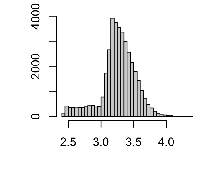
Further, a handful of genes are expressed in only a very small number of cells. I filter out genes that are expressed in fewer than 10 cells:
par(mar = c(4,4,1,1))
x <- colSums(counts > 0)
j <- which(x >= 10)
counts <- counts[,j]
hist(log10(x),n = 64,xlab = "",ylab = "",main = "")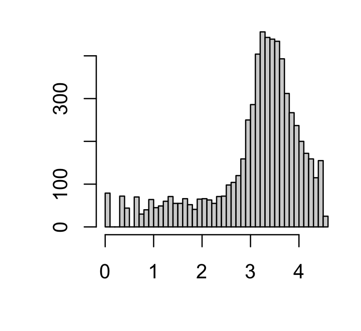
This gives the number of cells, the number of genes, and the proportion of counts that are nonzero after these filtering steps:
nrow(counts)
ncol(counts)
mean(counts > 0)
# [1] 33834
# [1] 6128
# [1] 0.1394832
And here is the number of cells in each of the 11 growth conditions:
table(sample_info$Condition)
#
# AmmoniumSulfate         CStarve       Glutamine     MinimalEtOH  MinimalGlucose
#             738             492            1644             449            1894
#         Proline            Urea             YPD      YPDDiauxic         YPDRapa
#             401             615           11037            3332           11805
#          YPEtOH
#            1427
To get an initial sense for the structure underlying the data, I generate a 2-d nonlinear embedding of the cells using UMAP. First, I transform the counts into “shifted log counts”:
a <- 1
s <- rowSums(counts)
s <- s/mean(s)
shifted_log_counts <- MatrixExtra::mapSparse(counts/(a*s),log1p)
Next, I project the cells onto the top 50 PCs:
set.seed(1)
U <- rsvd(shifted_log_counts,k = 50)$u
Then I run UMAP on the 50 PCs:
Y <- umap(U,n_neighbors = 20,metric = "cosine",min_dist = 0.3,
          n_threads = 8,verbose = FALSE)
sample_info$umap1 <- Y[,1]
sample_info$umap2 <- Y[,2]
UMAP with the cells colored by growth condition:
umap_colors <- c("#a6cee3","#1f78b4","#b2df8a","#33a02c","#fb9a99","#e31a1c",
                 "#fdbf6f","#ff7f00","#cab2d6","#6a3d9a","#ffff99")
p <- ggplot(sample_info,aes(x = umap1,y = umap2,color = Condition)) +
  geom_point(size = 1.5) +
  scale_color_manual(values = umap_colors) +
  labs(x = "UMAP 1",y = "UMAP 2") +
  theme_cowplot(font_size = 10)
print(p)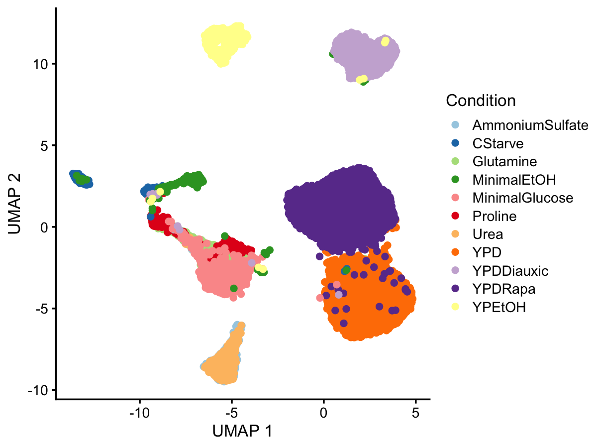
From this result, it is quite clear that the predominant structure corresponds to the different growth conditions. (This UMAP plot closely replicates Fig. 2B of the eLife paper.)
Finally, save the data and UMAP results to an .Rdata file for more convenient analysis in R:
save(list = c("sample_info","genes","counts"),file = "yeast.RData")
resaveRdaFiles("yeast.RData")
sessionInfo()
# R version 4.3.3 (2024-02-29)
# Platform: aarch64-apple-darwin20 (64-bit)
# Running under: macOS 15.5
#
# Matrix products: default
# BLAS:   /Library/Frameworks/R.framework/Versions/4.3-arm64/Resources/lib/libRblas.0.dylib
# LAPACK: /Library/Frameworks/R.framework/Versions/4.3-arm64/Resources/lib/libRlapack.dylib;  LAPACK version 3.11.0
#
# locale:
# [1] en_US.UTF-8/en_US.UTF-8/en_US.UTF-8/C/en_US.UTF-8/en_US.UTF-8
#
# time zone: America/Chicago
# tzcode source: internal
#
# attached base packages:
# [1] tools     stats     graphics  grDevices utils     datasets  methods
# [8] base
#
# other attached packages:
# [1] cowplot_1.1.3 ggplot2_3.5.2 uwot_0.2.3    rsvd_1.0.5    readr_2.1.5
# [6] Matrix_1.6-5
#
# loaded via a namespace (and not attached):
#  [1] sass_0.4.10         generics_0.1.4      stringi_1.8.7
#  [4] lattice_0.22-5      hms_1.1.3           digest_0.6.37
#  [7] magrittr_2.0.3      evaluate_1.0.4      grid_4.3.3
# [10] RColorBrewer_1.1-3  float_0.3-2         fastmap_1.2.0
# [13] rprojroot_2.0.4     workflowr_1.7.1     jsonlite_2.0.0
# [16] whisker_0.4.1       promises_1.3.3      scales_1.4.0
# [19] RhpcBLASctl_0.23-42 codetools_0.2-19    jquerylib_0.1.4
# [22] cli_3.6.5           rlang_1.1.6         crayon_1.5.3
# [25] RcppAnnoy_0.0.22    bit64_4.0.5         withr_3.0.2
# [28] cachem_1.1.0        yaml_2.3.10         parallel_4.3.3
# [31] tzdb_0.4.0          dplyr_1.1.4         httpuv_1.6.14
# [34] vctrs_0.6.5         R6_2.6.1            lifecycle_1.0.4
# [37] git2r_0.33.0        stringr_1.5.1       fs_1.6.6
# [40] bit_4.0.5           vroom_1.6.5         irlba_2.3.5.1
# [43] MatrixExtra_0.1.15  pkgconfig_2.0.3     pillar_1.11.0
# [46] bslib_0.9.0         later_1.4.2         gtable_0.3.6
# [49] glue_1.8.0          Rcpp_1.1.0          xfun_0.52
# [52] tibble_3.3.0        tidyselect_1.2.1    knitr_1.50
# [55] dichromat_2.0-0.1   farver_2.1.2        htmltools_0.5.8.1
# [58] labeling_0.4.3      rmarkdown_2.29      compiler_4.3.3