Structure plots and differential analysis of Buenrostro et al (2018) scATAC-seq data using fastTopics
Kaixuan Luo
Last updated: 2022-03-29
Checks: 7 0
Knit directory: scATACseq-topics/
This reproducible R Markdown analysis was created with workflowr (version 1.7.0). The Checks tab describes the reproducibility checks that were applied when the results were created. The Past versions tab lists the development history.
Great! Since the R Markdown file has been committed to the Git repository, you know the exact version of the code that produced these results.
Great job! The global environment was empty. Objects defined in the global environment can affect the analysis in your R Markdown file in unknown ways. For reproduciblity it's best to always run the code in an empty environment.
The command set.seed(20200729) was run prior to running the code in the R Markdown file. Setting a seed ensures that any results that rely on randomness, e.g. subsampling or permutations, are reproducible.
Great job! Recording the operating system, R version, and package versions is critical for reproducibility.
Nice! There were no cached chunks for this analysis, so you can be confident that you successfully produced the results during this run.
Great job! Using relative paths to the files within your workflowr project makes it easier to run your code on other machines.
Great! You are using Git for version control. Tracking code development and connecting the code version to the results is critical for reproducibility.
The results in this page were generated with repository version 181b83b. See the Past versions tab to see a history of the changes made to the R Markdown and HTML files.
Note that you need to be careful to ensure that all relevant files for the analysis have been committed to Git prior to generating the results (you can use wflow_publish or wflow_git_commit). workflowr only checks the R Markdown file, but you know if there are other scripts or data files that it depends on. Below is the status of the Git repository when the results were generated:
Ignored files:
    Ignored:    .DS_Store
    Ignored:    .Rhistory
    Ignored:    .Rproj.user/

Untracked files:
    Untracked:  .tmp.motifs
    Untracked:  analysis/motif_analysis_Buenrostro2018_v2.Rmd
    Untracked:  output/clustering-Cusanovich2018.rds
    Untracked:  paper/
    Untracked:  scripts/DA_Buenrostro2018_filteredpeaks.sbatch
    Untracked:  scripts/postfit_Buenrostro2018_filteredpeaks.sbatch
    Untracked:  scripts/postfit_Buenrostro2018_v2.sbatch

Unstaged changes:
    Modified:   analysis/assess_fits_Buenrostro2018_Chen2019pipeline.Rmd
    Modified:   analysis/clusters_Cusanovich2018_k13.Rmd
    Modified:   analysis/gene_analysis_Buenrostro2018_Chen2019pipeline.Rmd
    Modified:   analysis/gene_analysis_Cusanovich2018.Rmd
    Modified:   analysis/index.Rmd
    Modified:   analysis/motif_analysis_Buenrostro2018_Chen2019pipeline.Rmd
    Modified:   analysis/motif_analysis_Cusanovich2018.Rmd
    Modified:   analysis/plots_Cusanovich2018.Rmd
    Modified:   scripts/DA_analysis_Buenrostro2018_vsnull.R
    Modified:   scripts/analysis_Buenrostro2018_filteredpeaks.sh
Note that any generated files, e.g. HTML, png, CSS, etc., are not included in this status report because it is ok for generated content to have uncommitted changes.
These are the previous versions of the repository in which changes were made to the R Markdown (analysis/structureplot_DA_Buenrostro2018_filteredpeaks_k10.Rmd) and HTML (docs/structureplot_DA_Buenrostro2018_filteredpeaks_k10.html) files. If you've configured a remote Git repository (see ?wflow_git_remote), click on the hyperlinks in the table below to view the files as they were in that past version.
| File | Version | Author | Date | Message |
|---|---|---|---|---|
| Rmd | 181b83b | kevinlkx | 2022-03-29 | added structure plots for results with k = 8 and 9 |
Here we explore the structure in the Buenrostro et al (2018) scATAC-seq data inferred from the multinomial topic model.
Load packages and some functions used in this analysis.
library(fastTopics)
library(Matrix)
library(dplyr)
library(ggplot2)
library(cowplot)
library(plyr)
library(dplyr)
library(RColorBrewer)
library(DT)
library(reshape)
source("code/plots.R")
Load the data
Data downloaded from original paper.
Original data
data.dir <- "/project2/mstephens/kevinluo/scATACseq-topics/data/Buenrostro_2018/processed_data/"
load(file.path(data.dir, "Buenrostro_2018_binarized.RData"))
cat(sprintf("%d x %d counts matrix.\n",nrow(counts),ncol(counts)))
samples$cell <- rownames(samples)
samples$label <- as.factor(samples$label)
# 2034 x 465536 counts matrix.
Filtered out peaks with accessbility in fewer than 20 cells
i      <- which(colSums(counts) >= 20)
peaks  <- peaks[i,]
counts <- counts[,i]
cat(sprintf("After filtering, we have %d rows and %d columns left. \n",nrow(counts),ncol(counts)))
Load data after filtering peaks with accessbility in fewer than 20 cells
res.dir <- "/project2/mstephens/kevinluo/scATACseq-topics/output/Buenrostro_2018/binarized/filtered_peaks"
load(file.path(res.dir, "Buenrostro_2018_binarized_filtered.RData"))
cat(sprintf("%d x %d counts matrix.\n",nrow(counts),ncol(counts)))
samples$cell <- rownames(samples)
samples$label <- as.factor(samples$label)
# 2034 x 126719 counts matrix.
Topic model fit
K = 8
Load the K = 8 topic model fit
fit <- readRDS(file.path(res.dir, "/fit-Buenrostro2018-binarized-filtered-scd-ex-k=8.rds"))$fit
fit <- poisson2multinom(fit)
Structure plot
topic_colors <- c("darkorange","limegreen","magenta","gold","skyblue",
                  "darkblue","dodgerblue","darkmagenta")

set.seed(1)
# labels <- factor(samples$label, levels = c("HSC", "MPP", "CMP", "GMP", "mono", "MEP", "LMPP", "CLP", "pDC", "UNK"))

labels <- factor(samples$label, c("mono","pDC","MEP","HSC","MPP","CLP",
                                 "LMPP","CMP","GMP","UNK"))
structure_plot(fit,grouping = labels,colors = topic_colors,
               # topics = 1:10,
               gap = 20,perplexity = 50,verbose = FALSE)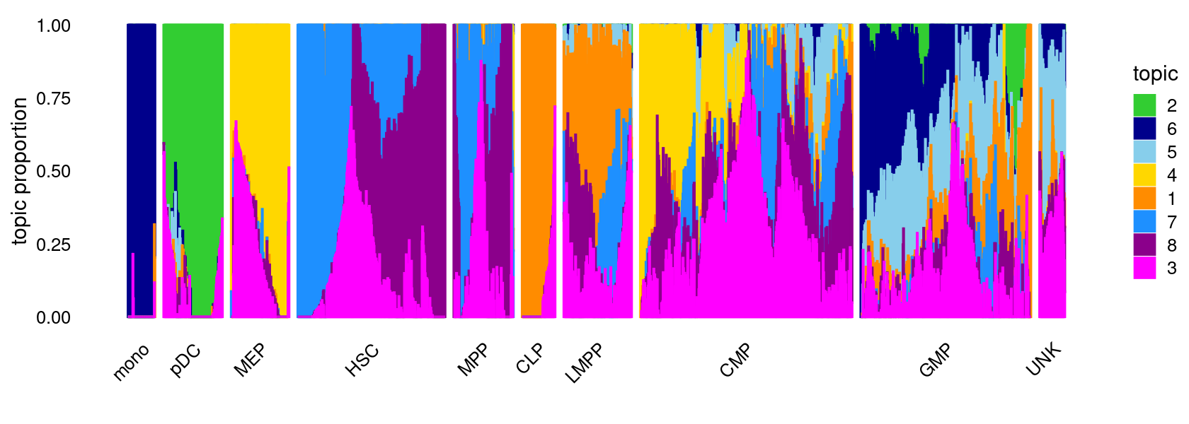
K = 9
Load the K = 9 topic model fit.
fit <- readRDS(file.path(res.dir, "/fit-Buenrostro2018-binarized-filtered-scd-ex-k=9.rds"))$fit
fit <- poisson2multinom(fit)
Structure plot
topic_colors <- c("darkorange","limegreen","magenta","gold","skyblue",
                  "darkblue","dodgerblue","darkmagenta","red")

set.seed(1)
# labels <- factor(samples$label, levels = c("HSC", "MPP", "CMP", "GMP", "mono", "MEP", "LMPP", "CLP", "pDC", "UNK"))

labels <- factor(samples$label, c("mono","pDC","MEP","HSC","MPP","CLP",
                                 "LMPP","CMP","GMP","UNK"))
structure_plot(fit,grouping = labels,colors = topic_colors,
               # topics = 1:10,
               gap = 20,perplexity = 50,verbose = FALSE)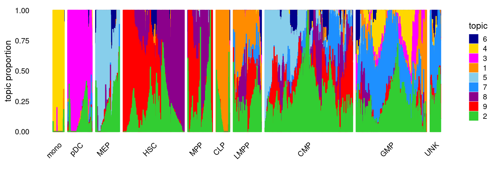
K = 10
Load the K = 10 topic model fit.
fit <- readRDS(file.path(res.dir, "/fit-Buenrostro2018-binarized-filtered-scd-ex-k=10.rds"))$fit
fit <- poisson2multinom(fit)
Structure plot
topic_colors <- c("darkorange","limegreen","magenta","gold","skyblue",
                  "darkblue","dodgerblue","darkmagenta","red","olivedrab")

set.seed(1)
# labels <- factor(samples$label, levels = c("HSC", "MPP", "CMP", "GMP", "mono", "MEP", "LMPP", "CLP", "pDC", "UNK"))

labels <- factor(samples$label, c("mono","pDC","MEP","HSC","MPP","CLP",
                                 "LMPP","CMP","GMP","UNK"))
structure_plot(fit,grouping = labels,colors = topic_colors,
               # topics = 1:10,
               gap = 20,perplexity = 50,verbose = FALSE)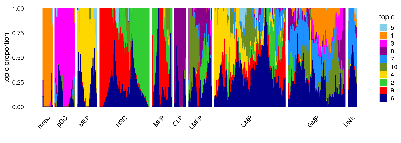
K-means clustering on topic proportions
Define clusters using k-means, and then create structure plot based on the clusters from k-means.
k-means clustering (using 12 clusters) on topic proportions
set.seed(1)
clusters <- factor(kmeans(fit$L,centers = 12,iter.max = 100)$cluster)
summary(clusters)

structure_plot(fit,grouping = clusters,colors = topic_colors,
               gap = 20,perplexity = 50,verbose = FALSE)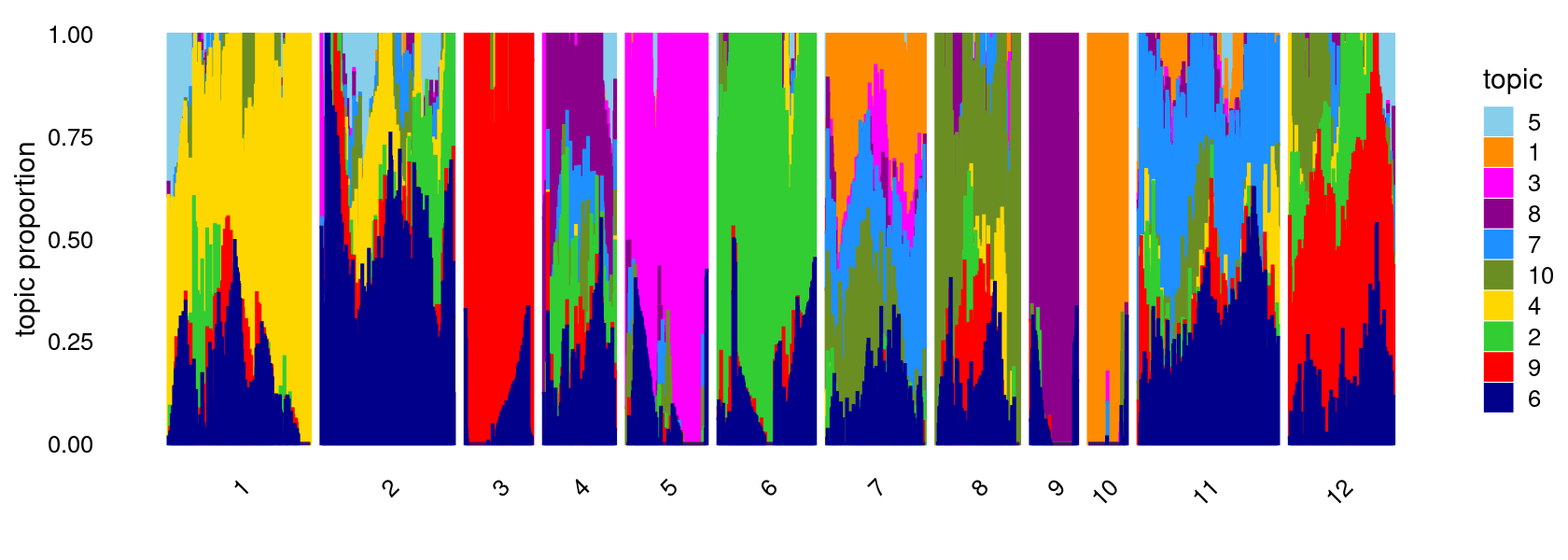
#   1   2   3   4   5   6   7   8   9  10  11  12
# 262 244 125 132 150 179 180 153  89  72 257 191
Differential accessibility (DA) analysis on topic modeling result with \(K = 10\)
DA analysis results without shrinkage (10000 MCMC iterations)
DA_dir <- "/project2/mstephens/kevinluo/scATACseq-topics/output/Buenrostro_2018/binarized/filtered_peaks/DAanalysis-Buenrostro2018-k=10"

DA_res <- readRDS(file.path(DA_dir, "DA_regions_topics_vsnull_noshrinkage_10000iters.rds"))
summary(DA_res)
#          Length  Class  Mode
# ar       1267190 -none- numeric
# est      1267190 -none- numeric
# postmean 1267190 -none- numeric
# lower    1267190 -none- numeric
# upper    1267190 -none- numeric
# z        1267190 -none- numeric
# lpval    1267190 -none- numeric
# svalue         1 -none- numeric
# lfsr           1 -none- numeric
# F        1267190 -none- numeric
# f0        126719 -none- numeric
Number of regions selected at different p-value cutoffs:
sig_regions <- matrix(NA, nrow = 10, ncol = 3)
colnames(sig_regions) <- c("p < 0.01", "p < 0.05", "p < 0.1")
rownames(sig_regions) <- paste("topic", 1:nrow(sig_regions))

for(k in 1:10){
  lpval <- DA_res$lpval[,k]
  pval <- 10^(-lpval)
  sig_regions[k, ] <- c(length(which(pval < 0.01)), length(which(pval < 0.05)), length(which(pval < 0.1)))
}

sig_regions
#          p < 0.01 p < 0.05 p < 0.1
# topic 1     15065    21923   28375
# topic 2     12633    20427   27623
# topic 3     16774    23671   29901
# topic 4     15825    20964   25905
# topic 5     15603    21209   24833
# topic 6      6986     9405   11438
# topic 7     14769    20177   24667
# topic 8     12989    20187   26041
# topic 9     15614    20703   24928
# topic 10     9455    14334   17737
Volcano plots for the regions
plots <- vector("list",10)
names(plots) <- 1:10

for (k in 1:10)
  plots[[k]] <- volcano_plot(DA_res, k, labels = rep("",nrow(DA_res$z)))
# lfsr is not available, probably because "shrink.method" was not set to "ash"; lfsr in plot should be ignored
# lfsr is not available, probably because "shrink.method" was not set to "ash"; lfsr in plot should be ignored
# lfsr is not available, probably because "shrink.method" was not set to "ash"; lfsr in plot should be ignored
# lfsr is not available, probably because "shrink.method" was not set to "ash"; lfsr in plot should be ignored
# lfsr is not available, probably because "shrink.method" was not set to "ash"; lfsr in plot should be ignored
# lfsr is not available, probably because "shrink.method" was not set to "ash"; lfsr in plot should be ignored
# lfsr is not available, probably because "shrink.method" was not set to "ash"; lfsr in plot should be ignored
# lfsr is not available, probably because "shrink.method" was not set to "ash"; lfsr in plot should be ignored
# lfsr is not available, probably because "shrink.method" was not set to "ash"; lfsr in plot should be ignored
# lfsr is not available, probably because "shrink.method" was not set to "ash"; lfsr in plot should be ignored
do.call(plot_grid,plots)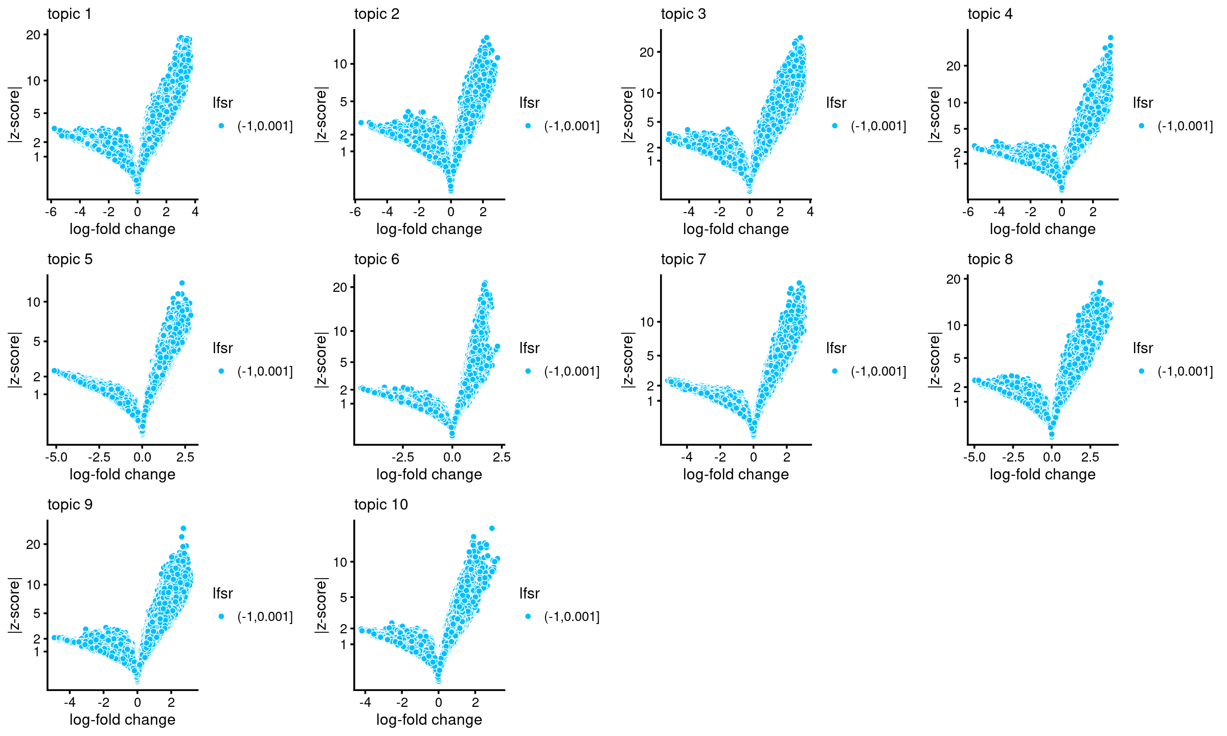
DA analysis results with "ash" shrinkage (10000 MCMC iterations)
DA_dir <- "/project2/mstephens/kevinluo/scATACseq-topics/output/Buenrostro_2018/binarized/filtered_peaks/DAanalysis-Buenrostro2018-k=10"

DA_res <- readRDS(file.path(DA_dir, "DA_regions_topics_vsnull_ash_10000iters.rds"))
summary(DA_res)

dim(DA_res$z)
#          Length  Class  Mode
# ar       1267190 -none- numeric
# est      1267190 -none- numeric
# postmean 1267190 -none- numeric
# lower    1267190 -none- numeric
# upper    1267190 -none- numeric
# z        1267190 -none- numeric
# lfsr     1267190 -none- numeric
# lpval          1 -none- numeric
# svalue   1267190 -none- numeric
# ash            3 ash    list
# F        1267190 -none- numeric
# f0        126719 -none- numeric
# [1] 126719     10
Number of regions selected at different lfsr cutoffs:
sig_regions <- matrix(NA, nrow = 10, ncol = 3)
colnames(sig_regions) <- c("lfsr < 0.01", "lfsr < 0.05", "lfsr < 0.1")
rownames(sig_regions) <- paste("topic", 1:nrow(sig_regions))

for(k in 1:10){
  lfsr <- DA_res$lfsr[,k]
  sig_regions[k, ] <- c(length(which(lfsr < 0.01)), length(which(lfsr < 0.05)), length(which(lfsr < 0.1)))
}

sig_regions
#          lfsr < 0.01 lfsr < 0.05 lfsr < 0.1
# topic 1        15066       21034      25515
# topic 2        11164       18536      24600
# topic 3        15139       20590      25533
# topic 4        14210       19177      23482
# topic 5        15240       22228      26977
# topic 6         6892        9588      11650
# topic 7        13505       19528      24046
# topic 8         9983       17102      22741
# topic 9        13028       18154      22778
# topic 10        6605       10974      14385
Volcano plots for the regions
plots <- vector("list",10)
names(plots) <- 1:10

for (k in 1:10)
  plots[[k]] <- volcano_plot(DA_res, k, labels = rep("",nrow(DA_res$z)))
do.call(plot_grid,plots)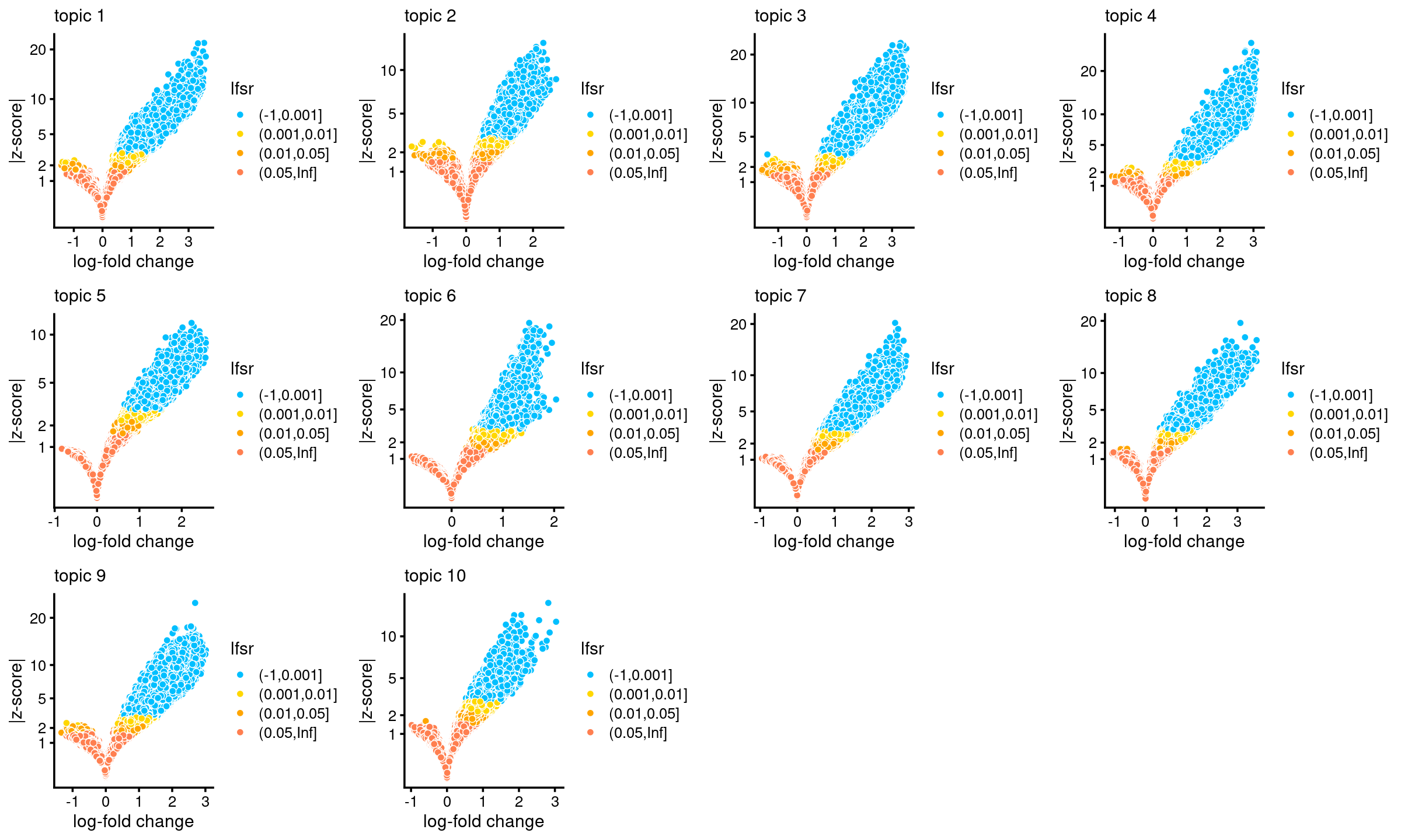
sessionInfo()
# R version 4.0.4 (2021-02-15)
# Platform: x86_64-pc-linux-gnu (64-bit)
# Running under: Scientific Linux 7.4 (Nitrogen)
#
# Matrix products: default
# BLAS/LAPACK: /software/openblas-0.3.13-el7-x86_64/lib/libopenblas_haswellp-r0.3.13.so
#
# locale:
#  [1] LC_CTYPE=en_US.UTF-8       LC_NUMERIC=C
#  [3] LC_TIME=en_US.UTF-8        LC_COLLATE=en_US.UTF-8
#  [5] LC_MONETARY=en_US.UTF-8    LC_MESSAGES=en_US.UTF-8
#  [7] LC_PAPER=en_US.UTF-8       LC_NAME=C
#  [9] LC_ADDRESS=C               LC_TELEPHONE=C
# [11] LC_MEASUREMENT=en_US.UTF-8 LC_IDENTIFICATION=C
#
# attached base packages:
# [1] stats     graphics  grDevices utils     datasets  methods   base
#
# other attached packages:
#  [1] reshape_0.8.8      DT_0.21            RColorBrewer_1.1-2 plyr_1.8.6
#  [5] cowplot_1.1.1      ggplot2_3.3.5      dplyr_1.0.8        Matrix_1.4-1
#  [9] fastTopics_0.6-97  workflowr_1.7.0
#
# loaded via a namespace (and not attached):
#  [1] mcmc_0.9-7         fs_1.5.2           progress_1.2.2     httr_1.4.2
#  [5] rprojroot_2.0.2    tools_4.0.4        bslib_0.3.1        utf8_1.2.2
#  [9] R6_2.5.1           irlba_2.3.5        uwot_0.1.11        DBI_1.1.2
# [13] lazyeval_0.2.2     colorspace_2.0-3   withr_2.5.0        tidyselect_1.1.2
# [17] prettyunits_1.1.1  processx_3.5.2     compiler_4.0.4     git2r_0.30.1
# [21] cli_3.2.0          quantreg_5.88      SparseM_1.81       plotly_4.10.0
# [25] labeling_0.4.2     sass_0.4.1         scales_1.1.1       SQUAREM_2021.1
# [29] quadprog_1.5-8     callr_3.7.0        pbapply_1.5-0      mixsqp_0.3-43
# [33] stringr_1.4.0      digest_0.6.29      rmarkdown_2.13     MCMCpack_1.6-1
# [37] pkgconfig_2.0.3    htmltools_0.5.2    highr_0.9          fastmap_1.1.0
# [41] invgamma_1.1       htmlwidgets_1.5.4  rlang_1.0.2        rstudioapi_0.13
# [45] farver_2.1.0       jquerylib_0.1.4    generics_0.1.2     jsonlite_1.8.0
# [49] magrittr_2.0.2     Rcpp_1.0.8.3       munsell_0.5.0      fansi_1.0.3
# [53] lifecycle_1.0.1    stringi_1.7.6      whisker_0.4        yaml_2.3.5
# [57] MASS_7.3-56        Rtsne_0.15         grid_4.0.4         parallel_4.0.4
# [61] promises_1.2.0.1   ggrepel_0.9.1      crayon_1.5.0       lattice_0.20-45
# [65] hms_1.1.1          knitr_1.37         ps_1.6.0           pillar_1.7.0
# [69] glue_1.6.2         evaluate_0.14      getPass_0.2-2      data.table_1.14.2
# [73] RcppParallel_5.1.5 vctrs_0.3.8        httpuv_1.6.5       MatrixModels_0.5-0
# [77] gtable_0.3.0       purrr_0.3.4        tidyr_1.2.0        assertthat_0.2.1
# [81] ashr_2.2-54        xfun_0.30          coda_0.19-4        later_1.3.0
# [85] viridisLite_0.4.0  truncnorm_1.0-8    tibble_3.1.6       ellipsis_0.3.2