Topic modeling analysis of Cusanovich et al (2018) data with k = 13 topics
Peter Carbonetto
Last updated: 2022-09-16
Checks: 7 0
Knit directory: scATACseq-topics/
This reproducible R Markdown analysis was created with workflowr (version 1.7.0). The Checks tab describes the reproducibility checks that were applied when the results were created. The Past versions tab lists the development history.
Great! Since the R Markdown file has been committed to the Git repository, you know the exact version of the code that produced these results.
Great job! The global environment was empty. Objects defined in the global environment can affect the analysis in your R Markdown file in unknown ways. For reproduciblity it’s best to always run the code in an empty environment.
The command set.seed(20200729) was run prior to running
the code in the R Markdown file. Setting a seed ensures that any results
that rely on randomness, e.g. subsampling or permutations, are
reproducible.
Great job! Recording the operating system, R version, and package versions is critical for reproducibility.
Nice! There were no cached chunks for this analysis, so you can be confident that you successfully produced the results during this run.
Great job! Using relative paths to the files within your workflowr project makes it easier to run your code on other machines.
Great! You are using Git for version control. Tracking code development and connecting the code version to the results is critical for reproducibility.
The results in this page were generated with repository version 1d2f32a. See the Past versions tab to see a history of the changes made to the R Markdown and HTML files.
Note that you need to be careful to ensure that all relevant files for
the analysis have been committed to Git prior to generating the results
(you can use wflow_publish or
wflow_git_commit). workflowr only checks the R Markdown
file, but you know if there are other scripts or data files that it
depends on. Below is the status of the Git repository when the results
were generated:
Ignored files:
    Ignored:    .DS_Store
    Ignored:    data/.DS_Store
    Ignored:    data/Buenrostro_2018/
    Ignored:    data/Cusanovich_2018/processed_data/Cusanovich_2018_Kidney.RData
    Ignored:    output/Buenrostro_2018/binarized/filtered_peaks/de-buenrostro2018-k=10-noshrink.RData
    Ignored:    output/Buenrostro_2018/binarized/filtered_peaks/fit-Buenrostro2018-binarized-filtered-scd-ex-k=10.rds
    Ignored:    output/Buenrostro_2018/binarized/filtered_peaks/fit-Buenrostro2018-binarized-filtered-scd-ex-k=8.rds
    Ignored:    output/Cusanovich_2018/.DS_Store
    Ignored:    output/Cusanovich_2018/fit-Cusanovich2018-scd-ex-k=13.rds
    Ignored:    output/Cusanovich_2018/tissues/.DS_Store
    Ignored:    output/Cusanovich_2018/tissues/de-cusanovich2018-kidney-k=10-noshrink.RData
    Ignored:    output/Cusanovich_2018/tissues/fit-Cusanovich2018-Kidney-scd-ex-k=10.rds
    Ignored:    output/Cusanovich_2018/tissues/gene-scores-cusanovich2018-kidney-k=10.RData
    Ignored:    scripts/seq_gene.md.gz

Untracked files:
    Untracked:  analysis/fit-Buenrostro2018-binarized-scd-ex-k=10.rds
    Untracked:  data/Buenrostro_2018_binarized.RData
    Untracked:  output/Buenrostro_2018/binarized/filtered_peaks/Buenrostro_2018_binarized_filtered.RData
    Untracked:  plots/
    Untracked:  scripts/fit-buenrostro-2018-k=8.rds
Note that any generated files, e.g. HTML, png, CSS, etc., are not included in this status report because it is ok for generated content to have uncommitted changes.
These are the previous versions of the repository in which changes were
made to the R Markdown (analysis/cusanovich2018_k13.Rmd)
and HTML (docs/cusanovich2018_k13.html) files. If you’ve
configured a remote Git repository (see ?wflow_git_remote),
click on the hyperlinks in the table below to view the files as they
were in that past version.
| File | Version | Author | Date | Message |
|---|---|---|---|---|
| Rmd | 1d2f32a | Peter Carbonetto | 2022-09-16 | workflowr::wflow_publish("analysis/cusanovich2018_k13.Rmd") |
| html | 99ebf60 | Peter Carbonetto | 2022-08-05 | Added text to beginning of cusanovich2018_k13 analysis. |
| Rmd | 4aca819 | Peter Carbonetto | 2022-08-05 | workflowr::wflow_publish("analysis/cusanovich2018_k13.Rmd", verbose = TRUE) |
| html | 5bcab84 | Peter Carbonetto | 2022-08-02 | Added NK cells to "other immune cells" in structure plot. |
| Rmd | b2af835 | Peter Carbonetto | 2022-08-02 | workflowr::wflow_publish("analysis/cusanovich2018_k13.Rmd", verbose = TRUE) |
| html | ffcfe12 | Peter Carbonetto | 2022-08-02 | Added notes to cusanovich2018_k13 analysis. |
| Rmd | d6d1bd1 | Peter Carbonetto | 2022-08-02 | workflowr::wflow_publish("analysis/cusanovich2018_k13.Rmd", verbose = TRUE) |
| html | cc5335a | Peter Carbonetto | 2022-08-02 | Revised the second structure plot. |
| Rmd | 0f830ba | Peter Carbonetto | 2022-08-02 | workflowr::wflow_publish("analysis/cusanovich2018_k13.Rmd", verbose = TRUE) |
| html | 9eff66b | Peter Carbonetto | 2022-08-01 | Added a second structure plot to the cusanovich2018_k13 analysis. |
| Rmd | 9e501cb | Peter Carbonetto | 2022-08-01 | workflowr::wflow_publish("analysis/cusanovich2018_k13.Rmd") |
| html | 05361f0 | Peter Carbonetto | 2022-08-01 | Made a couple small adjustments to the structure plot in the |
| Rmd | 37f3aeb | Peter Carbonetto | 2022-08-01 | workflowr::wflow_publish("analysis/cusanovich2018_k13.Rmd", verbose = TRUE) |
| html | 44d4987 | Peter Carbonetto | 2022-08-01 | Improved the structure plot in the cusanovich2018_k13 analysis. |
| Rmd | f62a0d1 | Peter Carbonetto | 2022-08-01 | workflowr::wflow_publish("analysis/cusanovich2018_k13.Rmd", verbose = TRUE) |
| html | 643af50 | Peter Carbonetto | 2022-08-01 | Build site. |
| Rmd | db1e9f0 | Peter Carbonetto | 2022-08-01 | workflowr::wflow_publish("analysis/cusanovich2018_k13.Rmd", verbose = TRUE) |
| html | 52d4663 | Peter Carbonetto | 2022-08-01 | First build of cusanovich2018_k13 analysis. |
| Rmd | cf89aa8 | Peter Carbonetto | 2022-08-01 | workflowr::wflow_publish("analysis/cusanovich2018_k13.Rmd", verbose = TRUE) |
Here we examine the structure inferred from the \(k = 13\) topic model fit the Cusanovich et al (2018) sci-ATAC-seq data.
Load the packages used in the analysis below.
library(Matrix)
library(fastTopics)
library(ggplot2)
Load the sample meta-data:
tissues <-
  c("BoneMarrow_62016","BoneMarrow_62216",
  "HeartA_62816","Kidney_62016","Testes_62016","SmallIntestine_62816",
  "LargeIntestineA_62816",
  "LargeIntestineB_62816","Liver_62016",
  "Lung1_62216","Lung2_62216",
  "Spleen_62016",
  "Thymus_62016","PreFrontalCortex_62216",
  "Cerebellum_62216","WholeBrainA_62216","WholeBrainA_62816")
load("data/Cusanovich_2018/processed_data/Cusanovich_2018_metadata_only.RData")
samples <- transform(samples,
                     tissue.replicate = factor(tissue.replicate,tissues))
Next load the \(k = 13\) multinomial topic model fit:
fit <- readRDS("output/Cusanovich_2018/fit-Cusanovich2018-scd-ex-k=13.rds")$fitThis Structure plot shows the cells arranged by tissue. Note that replicates were collected for four of the tissues (bone marrow, lung, small intestine, whole brain) in a second mouse.
set.seed(1)
topic_colors <- c("gold","royalblue","red","sienna","limegreen",
                  "plum","tomato","purple","cyan","forestgreen",
                  "darkblue","darkorange","lightgray")
topics <- c(1,2,5,6,9,11,4,10,8,3,7,12,13)
p1 <- structure_plot(fit,grouping = samples$tissue.replicate,gap = 30,n = 4000,
                     perplexity = 30,colors = topic_colors,topics = topics,
                     verbose = FALSE)
print(p1)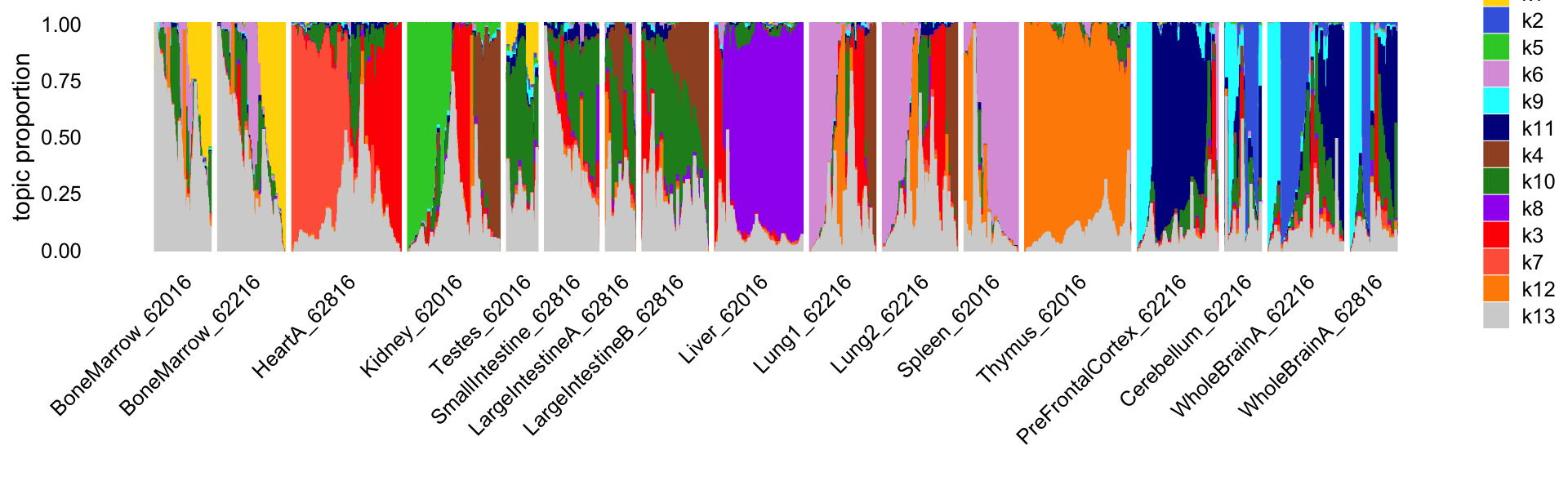
Reassuringly, the replicates show a very similar distribution of topics. Also reassuringly, some tissues are clearly distinguished by the topics (e.g., thymus), and similar tissues (e.g., small and large intenstine) share topics.
table(samples$tissue.replicate)
#
#       BoneMarrow_62016       BoneMarrow_62216           HeartA_62816
#                   4033                   4370                   7650
#           Kidney_62016           Testes_62016   SmallIntestine_62816
#                   6431                   2723                   4077
#  LargeIntestineA_62816  LargeIntestineB_62816            Liver_62016
#                   2281                   4805                   6167
#            Lung1_62216            Lung2_62216           Spleen_62016
#                   5122                   4874                   4020
#           Thymus_62016 PreFrontalCortex_62216       Cerebellum_62216
#                   7617                   5959                   2278
#      WholeBrainA_62216      WholeBrainA_62816
#                   5494                   3272
In this next Structure plot, we arrange the cells by the “major clusters” identified by Cusanovich et al (they used the Louvain community detection algorithm implemented in Seurat to identify these clusters).
cell_types <-
  c("Cardiomyocytes",
    "Astrocytes",
    "Oligodendrocytes",
    "Hepatocytes",
    "Podocytes",
    "Endothelial cells",
    "Neurons",
    "Purkinje cells",
    "Cerebellar granule cells",
    "T cells",
    "B cells",
    "Other immune cells",
    "Proximal tubule",
    "cluster 18",
    "Pneumocytes",
    "Enterocytes",
    "Erythroblasts",
    "Sperm",
    "Hematopoietic progenitors",
    "Collisions",
    "Unknown")
x <- samples$cell_label
x[x == "Activated B cells"] <- "B cells"
x[x == "Immature B cells"] <- "B cells"
x[x == "Ex. neurons CPN"] <- "Neurons"
x[x == "Ex. neurons SCPN"] <- "Neurons"
x[x == "Ex. neurons CThPN"] <- "Neurons"
x[x == "SOM+ Interneurons"] <- "Neurons"
x[x == "Inhibitory neurons"] <- "Neurons"
x[x == "Regulatory T cells"] <- "T cells"
x[x == "Endothelial I cells"] <- "Endothelial cells"
x[x == "Endothelial II cells"] <- "Endothelial cells"
x[x == "Endothelial I (glomerular)"] <- "Endothelial cells"
x[x == "Proximal tubule S3"] <- "Proximal tubule"
x[x == "Type I pneumocytes"] <- "Pneumocytes"
x[x == "Type II pneumocytes"] <- "Pneumocytes"
x[x == "Alveolar macrophages"] <- "Macrophages"
x[x == "Loop of henle"] <- "cluster 18"
x[x == "Distal convoluted tubule"] <- "cluster 18"
x[x == "Collecting duct"] <- "cluster 18"
x[x == "DCT/CD"] <- "cluster 18"
x[x == "Monocytes"] <- "Other immune cells"
x[x == "Dendritic cells"] <- "Other immune cells"
x[x == "Macrophages"] <- "Other immune cells"
x[x == "Microglia"] <- "Other immune cells"
x[x == "NK cells"] <- "Other immune cells"
samples <- transform(samples,
                     cell_label = factor(x,cell_types))
set.seed(1)
p2 <- structure_plot(fit,grouping = samples$cell_label,gap = 30,n = 4000,
                    perplexity = 30,colors = topic_colors,verbose = FALSE)
print(p2)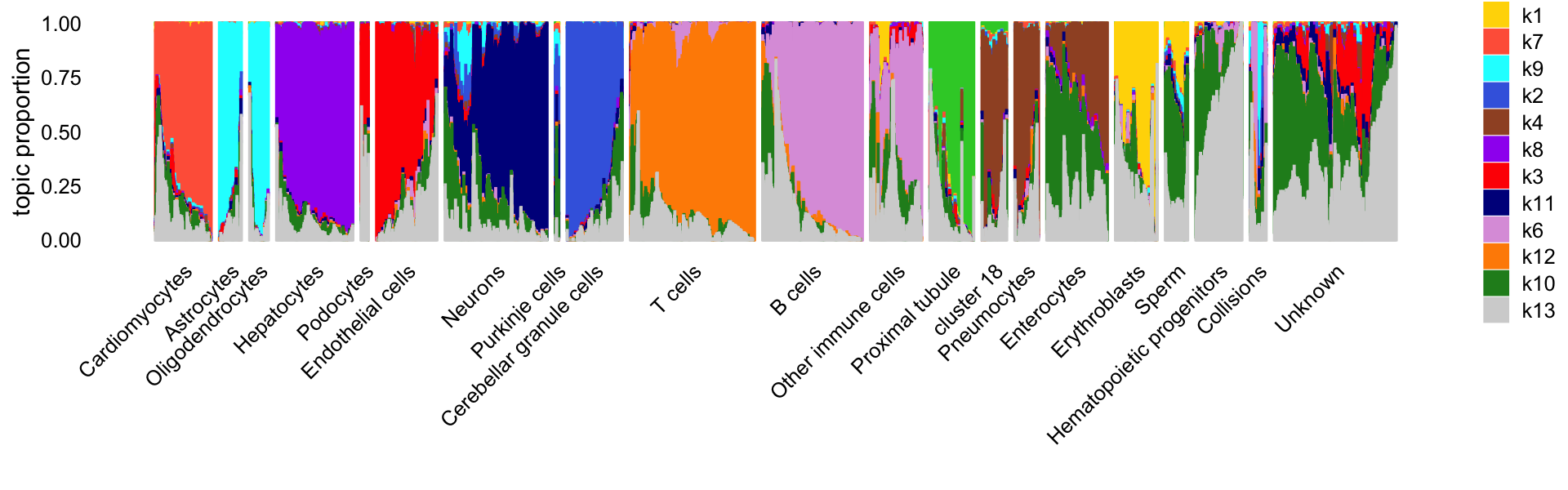
Clearly, the topics capture much of the high-level structure identified by the community detection algorithm.
table(samples$cell_label)
#
#            Cardiomyocytes                Astrocytes          Oligodendrocytes
#                      4076                      1666                      1558
#               Hepatocytes                 Podocytes         Endothelial cells
#                      5664                       498                      4523
#                   Neurons            Purkinje cells  Cerebellar granule cells
#                      7219                       320                      4099
#                   T cells                   B cells        Other immune cells
#                      9461                      6843                      4144
#           Proximal tubule                cluster 18               Pneumocytes
#                      3164                      1804                      1779
#               Enterocytes             Erythroblasts                     Sperm
#                      4783                      2811                      2089
# Hematopoietic progenitors                Collisions                   Unknown
#                      3425                      1218                     10029
sessionInfo()
# R version 3.6.2 (2019-12-12)
# Platform: x86_64-apple-darwin15.6.0 (64-bit)
# Running under: macOS Catalina 10.15.7
#
# Matrix products: default
# BLAS:   /Library/Frameworks/R.framework/Versions/3.6/Resources/lib/libRblas.0.dylib
# LAPACK: /Library/Frameworks/R.framework/Versions/3.6/Resources/lib/libRlapack.dylib
#
# locale:
# [1] en_US.UTF-8/en_US.UTF-8/en_US.UTF-8/C/en_US.UTF-8/en_US.UTF-8
#
# attached base packages:
# [1] stats     graphics  grDevices utils     datasets  methods   base
#
# other attached packages:
# [1] ggplot2_3.3.6      fastTopics_0.6-131 Matrix_1.4-2       workflowr_1.7.0
#
# loaded via a namespace (and not attached):
#  [1] mcmc_0.9-6         fs_1.5.2           progress_1.2.2     httr_1.4.2
#  [5] rprojroot_1.3-2    tools_3.6.2        backports_1.1.5    bslib_0.3.1
#  [9] utf8_1.1.4         R6_2.4.1           irlba_2.3.3        uwot_0.1.10
# [13] DBI_1.1.0          lazyeval_0.2.2     colorspace_1.4-1   withr_2.5.0
# [17] tidyselect_1.1.1   prettyunits_1.1.1  processx_3.5.2     compiler_3.6.2
# [21] git2r_0.29.0       quantreg_5.54      SparseM_1.78       plotly_4.9.2
# [25] labeling_0.3       sass_0.4.0         scales_1.1.0       SQUAREM_2017.10-1
# [29] quadprog_1.5-8     callr_3.7.0        pbapply_1.5-1      mixsqp_0.3-46
# [33] systemfonts_1.0.2  stringr_1.4.0      digest_0.6.23      rmarkdown_2.11
# [37] MCMCpack_1.4-5     pkgconfig_2.0.3    htmltools_0.5.2    fastmap_1.1.0
# [41] invgamma_1.1       highr_0.8          htmlwidgets_1.5.1  rlang_0.4.11
# [45] rstudioapi_0.13    jquerylib_0.1.4    generics_0.0.2     farver_2.0.1
# [49] jsonlite_1.7.2     dplyr_1.0.7        magrittr_2.0.1     Rcpp_1.0.8
# [53] munsell_0.5.0      fansi_0.4.0        lifecycle_1.0.0    stringi_1.4.3
# [57] whisker_0.4        yaml_2.2.0         MASS_7.3-51.4      Rtsne_0.15
# [61] grid_3.6.2         parallel_3.6.2     promises_1.1.0     ggrepel_0.9.1
# [65] crayon_1.4.1       lattice_0.20-38    cowplot_1.1.1      hms_1.1.0
# [69] knitr_1.37         ps_1.6.0           pillar_1.6.2       glue_1.4.2
# [73] evaluate_0.14      getPass_0.2-2      data.table_1.12.8  RcppParallel_5.1.5
# [77] vctrs_0.3.8        httpuv_1.5.2       MatrixModels_0.4-1 gtable_0.3.0
# [81] purrr_0.3.4        tidyr_1.1.3        assertthat_0.2.1   ashr_2.2-54
# [85] xfun_0.29          coda_0.19-3        later_1.0.0        ragg_0.3.1
# [89] viridisLite_0.3.0  truncnorm_1.0-8    tibble_3.1.3       ellipsis_0.3.2