Example 4: RSS-BVSR Fitting via Variational Bayes Methods
Xiang Zhu
Last updated: 2024-09-16
Checks: 2 0
Knit directory: rss/
This reproducible R Markdown analysis was created with workflowr (version 1.7.1). The Checks tab describes the reproducibility checks that were applied when the results were created. The Past versions tab lists the development history.
Great! Since the R Markdown file has been committed to the Git repository, you know the exact version of the code that produced these results.
Great! You are using Git for version control. Tracking code development and connecting the code version to the results is critical for reproducibility.
The results in this page were generated with repository version 941a146. See the Past versions tab to see a history of the changes made to the R Markdown and HTML files.
Note that you need to be careful to ensure that all relevant files for
the analysis have been committed to Git prior to generating the results
(you can use wflow_publish or
wflow_git_commit). workflowr only checks the R Markdown
file, but you know if there are other scripts or data files that it
depends on. Below is the status of the Git repository when the results
were generated:
Ignored files:
    Ignored:    .Rhistory
    Ignored:    .Rproj.user/
Note that any generated files, e.g. HTML, png, CSS, etc., are not included in this status report because it is ok for generated content to have uncommitted changes.
These are the previous versions of the repository in which changes were
made to the R Markdown (rmd/example_4.Rmd) and HTML
(docs/example_4.html) files. If you’ve configured a remote
Git repository (see ?wflow_git_remote), click on the
hyperlinks in the table below to view the files as they were in that
past version.
| File | Version | Author | Date | Message |
|---|---|---|---|---|
| html | bab3f58 | Xiang Zhu | 2020-06-24 | Build site. |
| html | 5efa0e9 | Xiang Zhu | 2020-06-24 | Build site. |
| Rmd | ee175ac | Xiang Zhu | 2020-06-24 | wflow_publish("rmd/example_4.Rmd") |
| html | cea3fa9 | Xiang Zhu | 2020-06-24 | Build site. |
| Rmd | db16ef7 | Xiang Zhu | 2020-06-24 | wflow_publish("rmd/example_4.Rmd") |
Overview
This example illustrates how to fit an RSS-BVSR model using variational Bayes (VB) approximation, and compares the results with previous work based on individual-level data, notably, Carbonetto and Stephens (2012). This example is closely related to Section “Connection with enrichment analysis of individual-level data” of Zhu and Stephens (2018).
Proposition 2.1 of Zhu and Stephens (2017) gives conditions under which regression likelihood based on individual-level data is equivalent to regression likelihood based on summary-level data. Under the same conditions, we can show that variational inferences based on individual-level data and summary-level data are also equivalent, in the sense that they have the same fix point iteration scheme and lower bound in variational approximations. See Supplementary Note of Zhu and Stephens (2018) for proofs. This example serves as a sanity check for our theoretical work.
The GWAS individual-level and summary-level data are simulated by enrich_datamaker.m,
which contains an enrichment signal of a target gene set. Specifically,
SNPs outside the target gene set are selected to be causal ones with
log10 odds ratio \(\theta_0\), whereas
SNPs inside this gene set are selected with a higher log10 odds ratio
\(\theta_0+\theta\) (\(\theta>0\)). For more details, see Supplementary
Figure 1 of Zhu and
Stephens (2018).
Next, we feed the simulated individual-level and summary-level data
to varbvs
and rss-varbvsr
respectively, and then compare the VB output from these two methods.
To reproduce results of Example 4, please please read the
step-by-step guide below and use example4.m.
Before running example4.m,
please first install the VB
subroutines of RSS Please find installation instructions here.
Step-by-step illustration
Step 1. Download
the input data genotype.mat and AH_chr16.mat
for the function enrich_datamaker.m. Please contact me if
you have trouble accessing these files1.
Step 2. Install the MATLAB implementation of varbvs. After
the installation, add varbvs to the search path as follows.
Step 3. Extract SNPs that inside the target gene set.
This step is where we need the input data AH_chr16.mat.
The index of SNPs inside the gene set is stored as
snps.
AH    = matfile('AH_chr16.mat');
H     = AH.H;                    % hypothesis matrix 3323x3160
A     = AH.A;                    % annotation matrix 12758x3323
paths = find(H(:,end));          % signal transduction (Biosystem, Reactome)
snps  = find(sum(A(:,paths),2)); % index of variants inside the pathway
Step 4. Simulate the enrichment dataset.
In addition to genotype.mat and
AH_chr16.mat, four more input variables are required in
order to run example4.m. You can provide them through
keyboard.
% set the number of replications
prompt = 'What is the number of replications? ';
Nrep   = input(prompt);

% set the genome-wide log-odds
prompt1 = 'What is the genome-wide log-odds? ';
theta0  = input(prompt1);

% set the log-fold enrichment
prompt2 = 'What is the log-fold enrichment? ';
theta   = input(prompt2);

% set the true pve
prompt3 = 'What is the pve (between 0 and 1)? ';
pve = input(prompt3);
With this in place, the data generation is all set.
for i = 1:Nrep
  myseed = 617 + i;

  % generate data under enrichment hypothesis
  [true_para,individual_data,summary_data] = enrich_datamaker(C,thetatype,pve,myseed,snps);

  ... ...

end
Step 5. Ensure that varbvs and
rss-varbvsr run in an almost identical environment.
We fix all the hyper-parameters as their true values, and give the same parameter initialization.
% fix all hyper-parameters as their true values
sigma   = true_para{4}^2;       % the true residual variance
sa      = 1/sigma;              % sa*sigma being the true prior variance of causal effects
sigb    = 1;                    % the true prior SD of causal effects
theta0  = thetatype(1);         % the true genome-wide log-odds (base 10)
theta   = thetatype(2);         % the true log-fold enrichment (base 10)

% initialize the variational parameters
rng(myseed, 'twister');
alpha0 = rand(p,1);
alpha0 = alpha0 ./ sum(alpha0);

rng(myseed+1, 'twister');
mu0 = randn(p,1);
Step 6. Run varbvs on the
individual-level genotypes and phenotypes.
The VB analysis involves two steps: first fitting the baseline model assuming no enrichment; second fitting the enrichment model assuming the gene set is enriched. We then calculate a Bayes factor (ratio of marginal likelihoods) for these two models, and use it to test whether the gene set is enriched for genetic associations.
fit_null = varbvs(X,[],y,[],'gaussian',options_n);
fit_gsea = varbvs(X,[],y,[],'gaussian',options_e);

bf_b = exp(fit_gsea.logw - fit_null.logw);
Step 7. Run rss-varbvsr on the
single-SNP association summary statistics.
Here we do not specify se and R as we
actually do in our real data analyses. Instead, we set their values such
that rss-varbvsr and varbvs are expected to
produce the same output. (This is because we want to verify our
mathematical proofs in silico.) Based on the proofs in Zhu and
Stephens (2018), we find that rss-varbvsr is equivalent
to varbvs if and only if
- the variance of phenotype is the same as residual variance
sigma.^2; - the input LD matrix
Ris the same as the sample correlation matrix of cohort genotypesX.
Reassuringly, these two assumptions are exactly the same assumptions in Proposition 2.1 of Zhu and Stephens (2017) that guarantees that the RSS likelihood is equivalent to the regression likelihood for individual-level data.
These two assumptions are implemented as follows.
% set the summary-level data for a perfect match b/t rss-varbvsr and varbvs
betahat = summary_data{1};
se      = sqrt(sigma ./ diag(X'*X));          % condition 1 for perfect matching
Si      = 1 ./ se(:);
R       = corrcoef(X);                        % condition 2 for perfect matching
SiRiS   = sparse(repmat(Si, 1, p) .* R .* repmat(Si', p, 1));
Now we perform the VB analysis of summary data via
rss-varbvsr.
[logw_nr,alpha_nr,mu_nr,s_nr] = rss_varbvsr(betahat,se,SiRiS,sigb,logodds_n,options);
[logw_er,alpha_er,mu_er,s_er] = rss_varbvsr(betahat,se,SiRiS,sigb,logodds_e,options);

bf_r = exp(logw_er-logw_nr);
Step 8. Compare VB output from varbvs
and rss-varbvsr.
Both varbvs and rss-varbvsr output an
estimated posterior distribution of \(\boldsymbol\beta\) (multiple regression
coefficients, or, multiple-SNP effect sizes). Specifically, both
estimated distributions have the following analytic form (Equations 6-7
in Carbonetto
and Stephens (2012)).
Hence, it suffices to compare the estimated variational parameters
[alpha, mu, s], and the estimated Bayes factors based on
the VB output. Below is the result when I only run
example4.m with one replication.
>> run example4.m
What is the number of replications? 1
What is the genome-wide log-odds? -4
What is the log-fold enrichment? 2
What is the pve (between 0 and 1)? 0.3
The log10 maximum absolute differences of [alpha, mu, s]
between varbvs and rss-varbvsr, under the
baseline model:
The log10 maximum absolute differences of [alpha, mu, s]
between varbvs and rss-varbvsr, under the
enrichment model:
The log10 Bayes factors estimated from varbvs and
rss-varbvsr are 4.0193 and 4.0193 respectively, and the
log10 relative difference between them is -6.8345.
More simulations
To see how example4.m behave on average, we need run
more replications. Below are the results from 100 replications.
>> run example4.m
What is the number of replications? 100
What is the genome-wide log-odds? -4
What is the log-fold enrichment? 2
What is the pve (between 0 and 1)? 0.3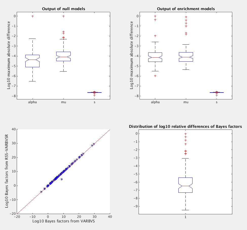
Footnotes:
- Currently these files are locked, since they contain individual-level genotypes from Wellcome Trust Case Control Consortium (WTCCC, https://www.wtccc.org.uk/). You need to get permission from WTCCC before we can share these files with you.