Example 3: RSS-BVSR with Various SE Vectors
Xiang Zhu
Last updated: 2024-09-16
Checks: 2 0
Knit directory: rss/
This reproducible R Markdown analysis was created with workflowr (version 1.7.1). The Checks tab describes the reproducibility checks that were applied when the results were created. The Past versions tab lists the development history.
Great! Since the R Markdown file has been committed to the Git repository, you know the exact version of the code that produced these results.
Great! You are using Git for version control. Tracking code development and connecting the code version to the results is critical for reproducibility.
The results in this page were generated with repository version 941a146. See the Past versions tab to see a history of the changes made to the R Markdown and HTML files.
Note that you need to be careful to ensure that all relevant files for
the analysis have been committed to Git prior to generating the results
(you can use wflow_publish or
wflow_git_commit). workflowr only checks the R Markdown
file, but you know if there are other scripts or data files that it
depends on. Below is the status of the Git repository when the results
were generated:
Ignored files:
    Ignored:    .Rhistory
    Ignored:    .Rproj.user/
Note that any generated files, e.g. HTML, png, CSS, etc., are not included in this status report because it is ok for generated content to have uncommitted changes.
These are the previous versions of the repository in which changes were
made to the R Markdown (rmd/example_3.Rmd) and HTML
(docs/example_3.html) files. If you’ve configured a remote
Git repository (see ?wflow_git_remote), click on the
hyperlinks in the table below to view the files as they were in that
past version.
| File | Version | Author | Date | Message |
|---|---|---|---|---|
| html | 2ac2497 | Xiang Zhu | 2024-07-03 | Build site. |
| Rmd | b7220ff | Xiang Zhu | 2024-07-03 | wflow_publish("rmd/example_3.Rmd") |
| html | bab3f58 | Xiang Zhu | 2020-06-24 | Build site. |
| html | 946a7a4 | Xiang Zhu | 2020-06-23 | Build site. |
| Rmd | 88d0b75 | Xiang Zhu | 2020-06-23 | wflow_publish("rmd/example_3.Rmd") |
Overview
This example illustrates the impact of different definitions of
standard error (se) on RSS. This example is closely related
to Section 2.1 of Zhu and Stephens
(2017).
The “simple” version of se is the standard error of
single-SNP effect estimate, which is often directly provided in GWAS
summary statistics database. The “rigorous” version of se
is used in theoretical derivations of RSS (see Section 2.4 of Zhu and Stephens
(2017)), and it requires some basic calculations based on commonly
available summary data.
Specifically, the “simple” version of se is given by
\[ \hat{\sigma}_j^2 = (n{\bf X}_j^\prime {\bf X}_j)^{-1} \cdot ({\bf y}-{\bf X}_j\hat{\beta}_j)^\prime ({\bf y}-{\bf X}_j\hat{\beta}_j), \]
and the “rigorous” version is given by
\[ \hat{s}_j^2=(n{\bf X}_j^\prime {\bf X}_j)^{-1} \cdot ({\bf y}^\prime{\bf y}). \]
The relation between these two versions is as follows
\[ \hat{s}_j^2=\hat{\sigma}_j^2 + n^{-1}\cdot \hat{\beta}_j^2. \]
Note that \(\hat{s}_j^2\approx\hat{\sigma}_j^2\) when \(n\) is large and/or \(\hat{\beta}_j^2\) is small.
In practice, we find these two definitions differ negligibly, mainly
because i) recent GWAS have large sample size (\(n\), Nsnp) and small effect
sizes (\(\hat{\beta}_j\),
betahat) (Table 1 of Zhu and Stephens
(2017)); and ii) published summary data are often rounded to two
digits to further limit the possibility of identifiability (e.g. GIANT).
Hence, we speculate that using these two definitions of
se exchangeably would not produce severely different
results in practice. Below we verify this speculation by
simulations.
Here we use the same dataset in Example 1. Please contact me if you have trouble downloading the dataset.
To reproduce results of Example 3, please read the step-by-step guide
below and run example3.m.
Before running example3.m,
please first install the MCMC
subroutines of RSS. Please find installation instructions here.
Step-by-step illustration
Step 1. Define two types of se.
We let se_1 and se_2 denote the “simple”
and “rigorous” version respectively.
Before running MCMC, we first look at the difference between these
two versions of se. Below is the five-number
summary1 of the absolute difference between se_1
and se_2.
>> abs_diff = abs(se_1 - se_2);
>> disp(prctile(log10(abs_diff), 0:25:100)); % require stat toolbox
  -12.0442   -4.6448   -3.9987   -3.4803   -1.3246
To make this example as “hard” as possible for RSS, we do not round
se_1 and se_2 to 2 significant digits.
Step 2. Fit RSS-BVSR using two versions of
se.
[betasam_1, gammasam_1, hsam_1, logpisam_1, Naccept_1] = rss_bvsr(betahat, se_1, R, Nsnp, Ndraw, Nburn, Nthin);
[betasam_2, gammasam_2, hsam_2, logpisam_2, Naccept_2] = rss_bvsr(betahat, se_2, R, Nsnp, Ndraw, Nburn, Nthin);
Step 3. Compare the posterior output.
We can look at the posterior means of beta, and
posterior distributions of h, log(pi) and PVE
based on se_1 (blue) and se_2 (orange).
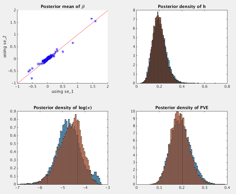
The PVE estimate (with 95% credible interval) is 0.1932, [0.1166,
0.2869] when using se_1, and it is 0.1896, [0.1162, 0.2765]
when using se_2.
More simulations
The simulations in Section 2.3 of Zhu and Stephens
(2017) are essentially “replications” of the example above. The
simulated datasets for Section 2.3 are available as
rss_example1_simulations.tar.gz2.
After applying RSS methods to these simulated data, we obtain the
following results, where sigma_hat corresponds to
se_1, and s_hat corresponds to
se_2.
| PVE estimation |
|---|
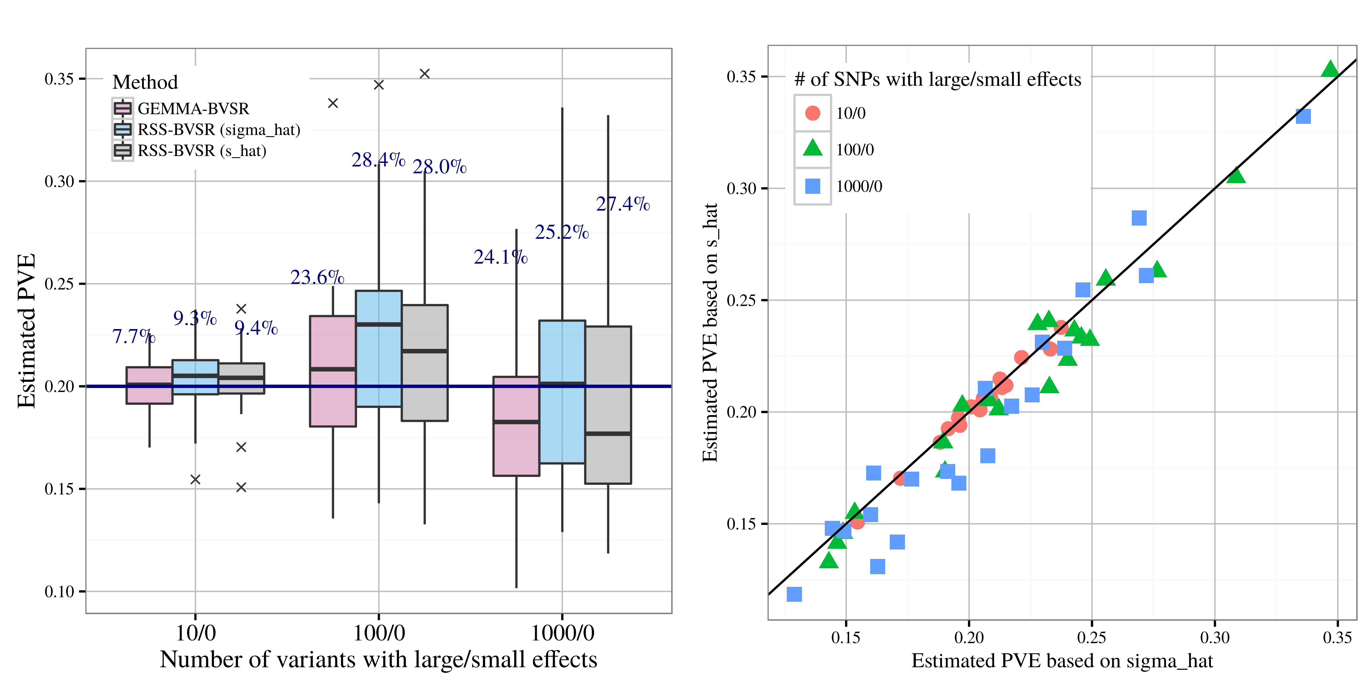 |
| Association detection |
|---|
 |
Footnotes:
The function
prctileused here requires the Statistics and Machine Learning Toolbox. Please see this commit (courtesy of Dr. Peter Carbonetto) if this required toolbox is not available in your environment.Currently these files are locked, since they contain individual-level genotypes from Wellcome Trust Case Control Consortium (WTCCC, https://www.wtccc.org.uk/). You need to get permission from WTCCC before we can share these files with you.