Example 5: Enrichment and prioritization analysis of GWAS summary statistics using RSS
Xiang Zhu
Last updated: 2020-06-24
Checks: 2 0
Knit directory: rss/
This reproducible R Markdown analysis was created with workflowr (version 1.6.2). The Checks tab describes the reproducibility checks that were applied when the results were created. The Past versions tab lists the development history.
Great! Since the R Markdown file has been committed to the Git repository, you know the exact version of the code that produced these results.
Great! You are using Git for version control. Tracking code development and connecting the code version to the results is critical for reproducibility.
The results in this page were generated with repository version 1e806af. See the Past versions tab to see a history of the changes made to the R Markdown and HTML files.
Note that you need to be careful to ensure that all relevant files for the analysis have been committed to Git prior to generating the results (you can use wflow_publish or wflow_git_commit). workflowr only checks the R Markdown file, but you know if there are other scripts or data files that it depends on. Below is the status of the Git repository when the results were generated:
Ignored files:
    Ignored:    .Rproj.user/
    Ignored:    .spelling
    Ignored:    examples/example5/.Rhistory
    Ignored:    examples/example5/Aseg_chr16.mat
    Ignored:    examples/example5/example5_simulated_data.mat
    Ignored:    examples/example5/example5_simulated_results.mat
    Ignored:    examples/example5/ibd2015_path2641_genes_results.mat

Untracked files:
    Untracked:  docs_old/

Unstaged changes:
    Modified:   rmd/_site.yml
Note that any generated files, e.g. HTML, png, CSS, etc., are not included in this status report because it is ok for generated content to have uncommitted changes.
These are the previous versions of the repository in which changes were made to the R Markdown (rmd/Example-5.Rmd) and HTML (docs/Example-5.html) files. If you’ve configured a remote Git repository (see ?wflow_git_remote), click on the hyperlinks in the table below to view the files as they were in that past version.
| File | Version | Author | Date | Message |
|---|---|---|---|---|
| html | c1eb295 | Xiang Zhu | 2020-06-24 | Build site. |
| Rmd | 9e93d5e | Xiang Zhu | 2020-06-24 | wflow_publish(“rmd/Example-5.Rmd”) |
Overview
This example illustrates how to perform enrichment and prioritization analysis of GWAS summary statistics based on variational Bayes (VB) inference of RSS-BVSR model. This example consists of:
Part A: analysis of a synthetic dataset used in simulation studies of Zhu and Stephens (2018);
Part B: analysis of published inflammatory bowel disease GWAS summary statistics (Liu et al, 2015) and a gene set named “IL23-mediated signaling events” (Pathway Commons 2, PID, 37 genes).
Part A provides a quick view of how RSS works in enrichment and prioritization analysis. Part B illustrates the actual data analyses performed in Zhu and Stephens (2018).
Details
The following figure provides a schematic overview of the method.
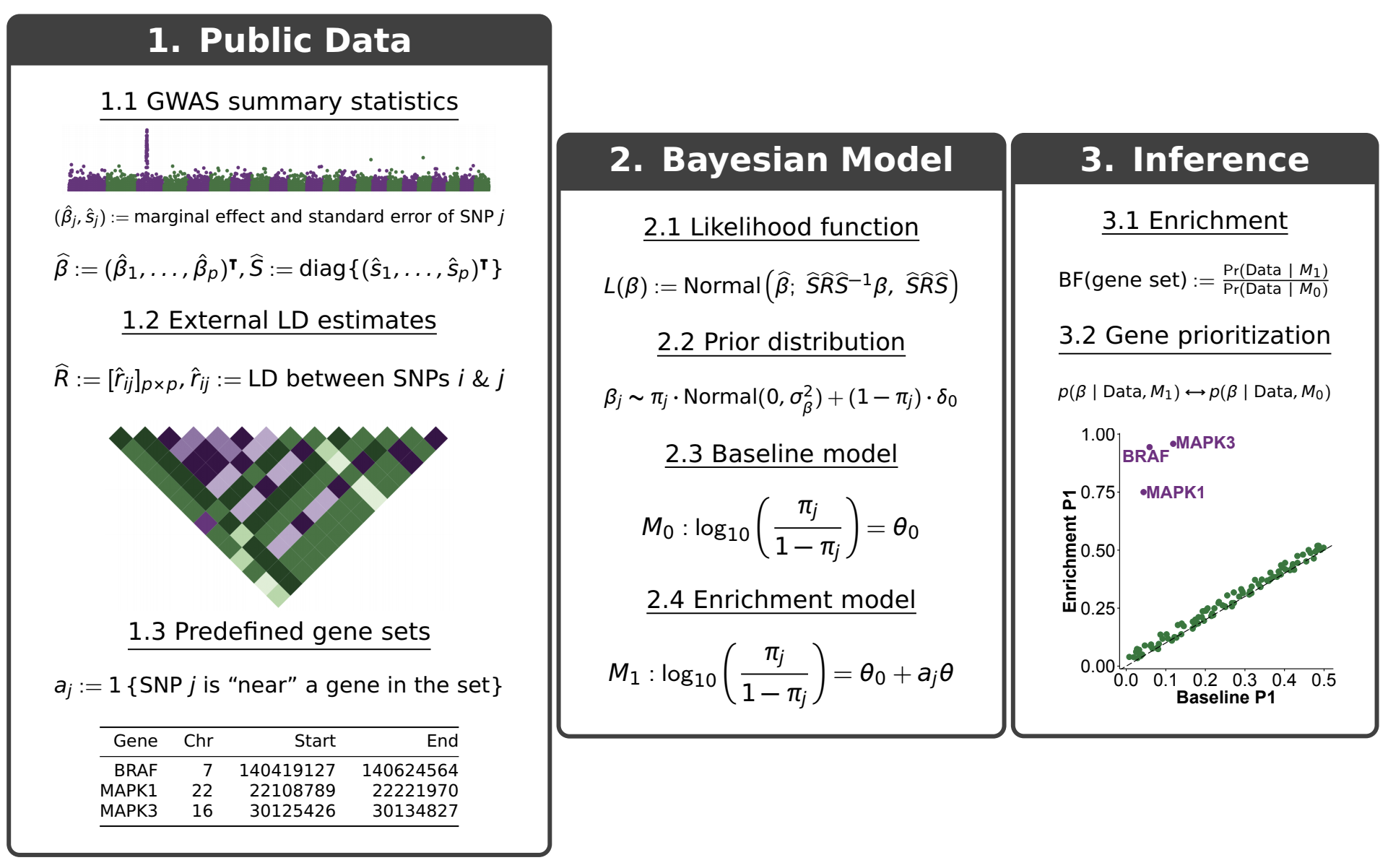
As shown above, RSS fits two models for the enrichment and prioritization analysis.
Baseline model (\(M_0\)): SNPs across the whole genome are equally likely to be associated with the phenotype of interest.
Enrichment model (\(M_1\)): SNPs “inside” a gene set are more likely (i.e. “enriched”) to be associated with a target phenotype than remaining SNPs.
If the gene set is truly enriched, then the observed GWAS data should show more support for the enrichment over baseline model, that is, yielding a larger Bayes factor (BF).
In addition to identifying enrichments, RSS also automatically prioritizes loci within an enriched set by comparing the posterior distributions of genetic effects (\(\beta\)) under \(M_0\) and \(M_1\). Here we summarize the posterior of beta as \(P_1\), the posterior probability that at least one SNP in a locus is trait-associated. Differences between \(P_1\) estimated under \(M_0\) and \(M_1\) reflect the influence of enrichment on genetic associations, which can help identify new trait-associated genes.
The key difference between RSS and previous work, notably, Carbonetto and Stephens (2013), is that RSS uses publicly available GWAS summary data, rather than individual-level genotypes and phenotypes. To perform similar analysis of GWAS individual-level data, please see https://github.com/pcarbo/bmapathway.
To reproduce results of Example 5, please use scripts in the directory example5. Before running the scripts, please make sure the VB subroutines of RSS are installed. Please find installation instructions here. It is advisable to go through the simulated example (Part A) before diving into the real data example (Part B).